Tkinter Increase Drawing Speed Images

Introduction

Overview

Teaching: 5 min
Exercises: 0 min

Questions

• What sort of scientific questions can we answer with image processing / computer vision?

• What are morphometric problems?

• What are colorimetric problems?

Objectives

• Recognize scientific questions that could be solved with image processing / computer vision.

• Recognize morphometric problems (those dealing with the number, size, or shape of the objects in an image).

• Recognize colorimetric problems (those dealing with the analysis of the color or the objects in an image).

We can use relatively simple image processing and computer vision techniques in Python, using the skimage library. With careful experimental design, a digital camera or a flatbed scanner, in conjunction with some Python code, can be a powerful instrument in answering many different kinds of problems. Consider the following two types of problems that might be of interest to a scientist.

Morphometrics

Morphometrics involves counting the number of objects in an image, analyzing the size of the objects, or analyzing the shape of the objects. For example, we might be interested automatically counting the number of bacterial colonies growing in a Petri dish, as shown in this image:

We could use image processing to find the colonies, count them, and then highlight their locations on the original image, resulting in an image like this:

Colorimetrics

Colorimetrics involves analyzing the color of objects in an image. For example, consider this video of a titrant being added to an analyte (click on the image to see the video):

We could use image processing to look at the color of the solution, and determine when the titration is complete. This graph shows how the three component colors (red, green, and blue) of the solution change over time; the change in the solution's color is obvious.

Why write a program to do that?

Note that you can easily manually count the number of bacteria colonies shown in the morphometric example above. Why should we learn how to write a Python program to do a task we could easily perform with our own eyes? There are at least two reasons to learn how to perform tasks like these with Python and skimage:

1. What if there are many more bacteria colonies in the Petri dish? For example, suppose the image looked like this:

   

   Manually counting the colonies in that image would present more of a challenge. A Python program using skimage could count the number of colonies more accurately, and much more quickly, than a human could.

2. What if you have hundreds, or thousands, of images to consider? Imagine having to manually count colonies on several thousand images like those above. A Python program using skimage could move through all of the images in seconds; how long would a graduate student require to do the task? Which process would be more accurate and repeatable?

As you can see, the simple image processing / computer vision techniques you will learn during this workshop can be very valuable tools for scientific research.

As we move through this workshop, we will return to these sample problems several times, and you will solve each of these problems during the end-of-workshop challenges.

Let's get started, by learning some basics about how images are represented and stored digitally.

Key Points

• Simple Python and skimage (scikit-image) techniques can be used to solve genuine morphometric and colorimetric problems.

• Morphometric problems involve the number, shape, and / or size of the objects in an image.

• Colorimetric problems involve analyzing the color of the objects in an image.

---

Image Basics

Overview

Teaching: 20 min
Exercises: 5 min

Questions

• How are images represented in digital format?

Objectives

• Define the terms bit, byte, kilobyte, megabyte, etc.

• Explain how a digital image is composed of pixels.

• Explain the left-hand coordinate system used in digital images.

• Explain the RGB additive color model used in digital images.

• Explain the characteristics of the BMP, JPEG, and TIFF image formats.

• Explain the difference between lossy and lossless compression.

• Explain the advantages and disadvantages of compressed image formats.

• Explain what information could be contained in image metadata.

The images we see on hard copy, view with our electronic devices, or process with our programs are represented and stored in the computer as numeric abstractions, approximations of what we see with our eyes in the real world. Before we begin to learn how to process images with Python programs, we need to spend some time understanding how these abstractions work.

Bits and bytes

Before we talk specifically about images, we first need to understand how numbers are stored in a modern digital computer. When we think of a number, we do so using a decimal, or base-10 place-value number system. For example, a number like 659 is 6 × 10² + 5 × 10¹ + 9 × 10⁰. Each digit in the number is multiplied by a power of 10, based on where it occurs, and there are 10 digits that can occur in each position (0, 1, 2, 3, 4, 5, 6, 7, 8, 9).

In principle, computers could be constructed to represent numbers in exactly the same way. But, as it turns out, the electronic circuits inside a computer are much easier to construct if we restrict the numeric base to only two, versus 10. (It is easier for circuitry to tell the difference between two voltage levels than it is to differentiate between 10 levels.) So, values in a computer are stored using a binary, or base-2 place-value number system.

In this system, each symbol in a number is called a bit instead of a digit, and there are only two values for each bit (0 and 1). We might imagine a four-bit binary number, 1101. Using the same kind of place-value expansion as we did above for 659, we see that 1101 = 1 × 2³ + 1 × 2² + 0 × 2¹ + 1 × 2⁰, which if we do the math is 8 + 4 + 0 + 1, or 13 in decimal.

Internally, computers have a minimum number of bits that they work with at a given time: eight. A group of eight bits is called a byte. The amount of memory (RAM) and drive space our computers have is quantified by terms like Megabytes (MB), Gigabytes (GB), and Terabytes (TB). The following table provides more formal definitions for these terms.

Unit	Abbreviation	Size
Kilobyte	KB	1024 bytes
Megabyte	MB	1024 KB
Gigabyte	GB	1024 MB
Terabyte	TB	1024 GB

Pixels

It is important to realize that images are stored as rectangular arrays of hundreds, thousands, or millions of discrete "picture elements," otherwise known as pixels. Each pixel can be thought of as a single square point of colored light.

For example, consider this image of a maize seedling, with a square area designated by a red box:

Now, if we zoomed in close enough to see the pixels in the red box, we would see something like this:

Note that each square in the enlarged image area – each pixel – is all one color, but that each pixel can have a different color from its neighbors. Viewed from a distance, these pixels seem to blend together to form the image we see.

Coordinate system

When we process images, we can access, examine, and / or change the color of any pixel we wish. To do this, we need some convention on how to access pixels individually; a way to give each one a name, or an address of a sort.

The most common manner to do this, and the one we will use in our programs, is to assign a modified Cartesian coordinate system to the image. The coordinate system we usually see in mathematics has a horizontal x-axis and a vertical y-axis, like this:

The modified coordinate system used for our images will have only positive coordinates, the origin will be in the upper left corner instead of the center, and y coordinate values will get larger as they go down instead of up, like this:

This is called a left-hand coordinate system. If you hold your left hand in front of your face and point your thumb at the floor, your extended index finger will correspond to the x-axis while your thumb represents the y-axis.

Until you have worked with images for a while, the most common mistake that you will make with coordinates is to forget that y coordinates get larger as they go down instead of up as in a normal Cartesian coordinate system.

Color model

Digital images use some color model to create a broad range of colors from a small set of primary colors. Although there are several different color models that are used for images, the most commonly occurring one is the RGB (Red, Green, Blue) model.

The RGB model is an additive color model, which means that the primary colors are mixed together to form other colors. In the RGB model, the primary colors are red, green, and blue – thus the name of the model. Each primary color is often called a channel.

Most frequently, the amount of the primary color added is represented as an integer in the closed range [0, 255]. Therefore, there are 256 discrete amounts of each primary color that can be added to produce another color. The number of discrete amounts of each color, 256, corresponds to the number of bits used to hold the color channel value, which is eight (2⁸=256). Since we have three channels, this is called 24-bit color depth.

Any particular color in the RGB model can be expressed by a triplet of integers in [0, 255], representing the red, green, and blue channels, respectively. A larger number in a channel means that more of that primary color is present.

Thinking about RGB colors (5 min)

Suppose that we represent colors as triples (r, g, b), where each of r, g, and b is an integer in [0, 255]. What colors are represented by each of these triples? (Try to answer these questions without reading further.)

1. (255, 0, 0)
2. (0, 255, 0)
3. (0, 0, 255)
4. (255, 255, 255)
5. (0, 0, 0)
6. (128, 128, 128)

Solution

1. (255, 0, 0) represents red, because the red channel is maximized, while the other two channels have the minimum values.
2. (0, 255, 0) represents green.
3. (0, 0, 255) represents blue.
4. (255, 255, 255) is a little harder. When we mix the maximum value of all three color channels, we see the color white.
5. (0, 0, 0) represents the absence of all color, or black.
6. (128, 128, 128) represents a medium shade of gray. Note that the 24-bit RGB color model provides at least 254 shades of gray, rather than only fifty.

Note that the RGB color model may run contrary to your experience, especially if you have mixed primary colors of paint to create new colors. In the RGB model, the lack of any color is black, while the maximum amount of each of the primary colors is white. With physical paint, we might start with a white base, and then add differing amounts of other paints to produce a darker shade.

After completing the previous challenge, we can look at some further examples of 24-bit RGB colors, in a visual way. The image in the next challenge shows some color names, their 24-bit RGB triplet values, and the color itself.

RGB color table (optional, not included in timing)

We cannot really provide a complete table. To see why, answer this question: How many possible colors can be represented with the 24-bit RGB model?

Solution

There are 24 total bits in an RGB color of this type, and each bit can be on or off, and so there are 2²⁴ = 16,777,216 possible colors with our additive, 24-bit RGB color model.

Although 24-bit color depth is common, there are other options. We might have 8-bit color (3 bits for red and green, but only 2 for blue, providing 8 × 8 × 4 = 256 colors) or 16-bit color (4 bits for red, green, and blue, plus 4 more for transparency, providing 16 × 16 × 16 = 4096 colors), for example. There are color depths with more than eight bits per channel, but as the human eye can only discern approximately 10 million different colors, these are not often used.

If you are using an older or inexpensive laptop screen or LCD monitor to view images, it may only support 18-bit color, capable of displaying 64 × 64 × 64 = 262,144 colors. 24-bit color images will be converted in some manner to 18-bit, and thus the color quality you see will not match what is actually in the image.

We can combine our coordinate system with the 24-bit RGB color model to gain a conceptual understanding of the images we will be working with. An image is a rectangular array of pixels, each with its own coordinate. Each pixel in the image is a square point of colored light, where the color is specified by a 24-bit RGB triplet. Such an image is an example of raster graphics.

Image formats

Although the images we will manipulate in our programs are conceptualized as rectangular arrays of RGB triplets, they are not necessarily created, stored, or transmitted in that format. There are several image formats we might encounter, and we should know the basics of at least of few of them. Some formats we might encounter, and their file extensions, are shown in this table:

Format	Extension
Device-Independent Bitmap (BMP)	.bmp
Joint Photographic Experts Group (JPEG)	.jpg or .jpeg
Tagged Image File Format (TIFF)	.tif or .tiff

BMP

The file format that comes closest to our preceding conceptualization of images is the Device-Independent Bitmap, or BMP, file format. BMP files store raster graphics images as long sequences of binary-encoded numbers that specify the color of each pixel in the image. Since computer files are one-dimensional structures, the pixel colors are stored one row at a time. That is, the first row of pixels (those with y-coordinate 0) are stored first, followed by the second row (those with y-coordinate 1), and so on. Depending on how it was created, a BMP image might have 8-bit, 16-bit, or 24-bit color depth.

24-bit BMP images have a relatively simple file format, can be viewed and loaded across a wide variety of operating systems, and have high quality. However, BMP images are not compressed, resulting in very large file sizes for any useful image resolutions.

The idea of image compression is important to us for two reasons: first, compressed images have smaller file sizes, and are therefore easier to store and transmit; and second, compressed images may not have as much detail as their uncompressed counterparts, and so our programs may not be able to detect some important aspect if we are working with compressed images. Since compression is important to us, we should take a brief detour and discuss the concept.

Image compression

Let's begin our discussion of compression with a simple challenge.

BMP image size (optional, not included in timing)

Imagine that we have a fairly large, but very boring image: a 5,000 × 5,000 pixel image composed of nothing but white pixels. If we used an uncompressed image format such as BMP, with the 24-bit RGB color model, how much storage would be required for the file?

Solution

In such an image, there are 5,000 × 5,000 = 25,000,000 pixels, and 24 bits for each pixel, leading to 25,000,000 × 24 = 600,000,000 bits, or 75,000,000 bytes (71.5MB). That is quite a lot of space for a very uninteresting image!

Since image files can be very large, various compression schemes exist for saving (approximately) the same information while using less space. These compression techniques can be categorized as lossless or lossy.

Lossless compression

In lossless image compression, we apply some algorithm (i.e., a computerized procedure) to the image, resulting in a file that is significantly smaller than the uncompressed BMP file equivalent would be. Then, when we wish to load and view or process the image, our program reads the compressed file, and reverses the compression process, resulting in an image that is identical to the original. Nothing is lost in the process – hence the term "lossless."

The general idea of lossless compression is to somehow detect long patterns of bytes in a file that are repeated over and over, and then assign a smaller bit pattern to represent the longer sample. Then, the compressed file is made up of the smaller patterns, rather than the larger ones, thus reducing the number of bytes required to save the file. The compressed file also contains a table of the substituted patterns and the originals, so when the file is decompressed it can be made identical to the original before compression.

To provide you with a concrete example, consider the 71.5 MB white BMP image discussed above. When put through the zip compression utility on Microsoft Windows, the resulting .zip file is only 72 KB in size! That is, the .zip version of the image is three orders of magnitude smaller than the original, and it can be decompressed into a file that is byte-for-byte the same as the original. Since the original is so repetitious – simply the same color triplet repeated 25,000,000 times – the compression algorithm can dramatically reduce the size of the file.

If you work with .zip or .gz archives, you are dealing with lossless compression.

Lossy compression

Lossy compression takes the original image and discards some of the detail in it, resulting in a smaller file format. The goal is to only throw away detail that someone viewing the image would not notice. Many lossy compression schemes have adjustable levels of compression, so that the image creator can choose the amount of detail that is lost. The more detail that is sacrificed, the smaller the image files will be – but of course, the detail and richness of the image will be lower as well.

This is probably fine for images that are shown on Web pages or printed off on 4 × 6 photo paper, but may or may not be fine for scientific work. You will have to decide whether the loss of image quality and detail are important to your work, versus the space savings afforded by a lossy compression format.

It is important to understand that once an image is saved in a lossy compression format, the lost detail is just that – lost. I.e., unlike lossless formats, given an image saved in a lossy format, there is no way to reconstruct the original image in a byte-by-byte manner.

JPEG

JPEG images are perhaps the most commonly encountered digital images today. JPEG uses lossy compression, and the degree of compression can be tuned to your liking. It supports 24-bit color depth, and since the format is so widely used, JPEG images can be viewed and manipulated easily on all computing platforms.

Examining actual image sizes (optional, not included in timing)

Let us see the effects of image compression on image size with actual images. Open a terminal and navigate to the Desktop/workshops/image-processing/02-image-basics directory. This directory contains a simple program, ws.py that creates a square white image of a specified size, and then saves it as a BMP and as a JPEG image.

To create a 5,000 x 5,000 white square, execute the program by typing python ws.py 5000 and then hitting enter. Then, examine the file sizes of the two output files, ws.bmp and ws.jpg. Does the BMP image size match our previous prediction? How about the JPEG?

Solution

The BMP file, ws.bmp, is 75,000,054 bytes, which matches our prediction very nicely. The JPEG file, ws.jpg, is 392,503 bytes, two orders of magnitude smaller than the bitmap version.

Comparing lossless versus lossy compression (optional, not included in timing)

Let us see a hands-on example of lossless versus lossy compression. Once again, open a terminal and navigate to the Desktop/workshops/image-processing/02-image-basics directory. The two output images, ws.bmp and ws.jpg, should still be in the directory, along with another image, tree.jpg.

We can apply lossless compression to any file by using the zip command. Recall that the ws.bmp file contains 75,000,054 bytes. Apply lossless compression to this image by executing the following command: zip ws.zip ws.bmp. This command tells the computer to create a new compressed file, ws.zip, from the original bitmap image. Execute a similar command on the tree JPEG file: zip tree.zip tree.jpg.

Having created the compressed file, use the ls -al command to display the contents of the directory. How big are the compressed files? How do those compare to the size of ws.bmp and tree.jpg? What can you conclude from the relative sizes?

Solution

Here is a partial directory listing, showing the sizes of the relevant files there:

-rw-rw-r– 1 diva diva 154344 Jun 18 08:32 tree.jpg

-rw-rw-r– 1 diva diva 146049 Jun 18 08:53 tree.zip

-rw-rw-r– 1 diva diva 75000054 Jun 18 08:51 ws.bmp

-rw-rw-r– 1 diva diva 72986 Jun 18 08:53 ws.zip

We can see that the regularity of the bitmap image (remember, it is a 5,000 x 5,000 pixel image containing only white pixels) allows the lossless compression scheme to compress the file quite effectively. On the other hand, compressing tree.jpg does not create a much smaller file; this is because the JPEG image was already in a compressed format.

Here is an example showing how JPEG compression might impact image quality. Consider this image of several maize seedlings (scaled down here from 11,339 × 11,336 pixels in order to fit the display).

Now, let us zoom in and look at a small section of the label in the original, first in the uncompressed format:

Here is the same area of the image, but in JPEG format. We used a fairly aggressive compression parameter to make the JPEG, in order to illustrate the problems you might encounter with the format.

The JPEG image is of clearly inferior quality. It has less color variation and noticeable pixelation. Quality differences become even more marked when one examines the color histograms for each image. A histogram shows how often each color value appears in an image. The histograms for the uncompressed (left) and compressed (right) images are shown below:

We we learn how to make histograms such as these later on in the workshop. The differences in the color histograms are even more apparent than in the images themselves; clearly the colors in the JPEG image are different from the uncompressed version.

If the quality settings for your JPEG images are high (and the compression rate therefore relatively low), the images may be of sufficient quality for your work. It all depends on how much quality you need, and what restrictions you have on image storage space. Another consideration may be where the images are stored. For example, if your images are stored in the cloud and therefore must be downloaded to your system before you use them, you may wish to use a compressed image format to speed up file transfer time.

TIFF

TIFF images are popular with publishers, graphics designers, and photographers. TIFF images can be uncompressed, or compressed using either lossless or lossy compression schemes, depending on the settings used, and so TIFF images seem to have the benefits of both the BMP and JPEG formats. The main disadvantage of TIFF images (other than the size of images in the uncompressed version of the format) is that they are not universally readable by image viewing and manipulation software.

JPEG and TIFF images support the inclusion of metadata in images. Metadata is textual information that is contained within an image file. Metadata holds information about the image itself, such as when the image was captured, where it was captured, what type of camera was used and with what settings, etc. We normally don't see this metadata when we view an image, but programs exist that can allow us to view it if we wish to (see Accessing Metadata, below). The important thing to be aware of at this stage is that you cannot rely on the metadata of an image being preserved when you use software to process that image. The image processing library that we will use in the rest of this lesson, skimage, does not include metadata when saving new images. So remember: if metadata is important to you, take precautions to always preserve the original files.

Although skimage does not provide a way to display or explore the metadata associated with an image (and subsequently cannot preserve that metadata when modifying an image file), other software exists that can help you to do so, e.g. Fiji and ImageMagick. We recommend you explore these options if you really need to work with the metadata of your images.

Summary of image formats used in this lesson

The following table summarizes the characteristics of the BMP, JPEG, and TIFF image formats:

Format	Compression	Metadata	Advantages	Disadvantages
BMP	None	None	Universally viewable,	Large file sizes
			high quality
JPEG	Lossy	Yes	Universally viewable,	Detail may be lost
			smaller file size
TIFF	None, lossy,	Yes	High quality or	Not universally viewable
	or lossless		smaller file size

Key Points

• Digital images are represented as rectangular arrays of square pixels.

• Digital images use a left-hand coordinate system, with the origin in the upper left corner, the x-axis running to the right, and the y-axis running down.

• Most frequently, digital images use an additive RGB model, with eight bits for the red, green, and blue channels.

• Lossless compression retains all the details in an image, but lossy compression results in loss of some of the original image detail.

• BMP images are uncompressed, meaning they have high quality but also that their file sizes are large.

• JPEG images use lossy compression, meaning that their file sizes are smaller, but image quality may suffer.

• TIFF images can be uncompressed or compressed with lossy or lossless compression.

• Depending on the camera or sensor, various useful pieces of information may be stored in an image file, in the image metadata.

---

Image representation in skimage

Overview

Teaching: 70 min
Exercises: 50 min

Questions

• How are digital images stored in Python with the skimage computer vision library?

Objectives

• Explain how images are stored in NumPy arrays.

• Explain the order of the three color values in skimage images.

• Read, display, and save images using skimage.

• Resize images with skimage.

• Perform simple image thresholding with NumPy array operations.

• Explain why command-line parameters are useful.

• Extract sub-images using array slicing.

Now that we know a bit about computer images in general, let us turn to more details about how images are represented in the skimage open-source computer vision library.

Images are represented as NumPy arrays

In the Image Basics episode, we learned that images are represented as rectangular arrays of individually-colored square pixels, and that the color of each pixel can be represented as an RGB triplet of numbers. In skimage, images are stored in a manner very consistent with the representation from that episode. In particular, images are stored as three-dimensional NumPy arrays.

The rectangular shape of the array corresponds to the shape of the image, although the order of the coordinates are reversed. The "depth" of the array for an skimage image is three, with one layer for each of the three channels. The differences in the order of coordinates and the order of the channel layers can cause some confusion, so we should spend a bit more time looking at that.

When we think of a pixel in an image, we think of its (x, y) coordinates (in a left-hand coordinate system) like (113, 45) and its color, specified as a RGB triple like (245, 134, 29). In an skimage image, the same pixel would be specified with (y, x) coordinates (45, 113) and RGB color (245, 134, 29).

Let us take a look at this idea visually. Consider this image of a chair:

A visual representation of how this image is stored as a NumPy array is:

So, when we are working with skimage images, we specify the y coordinate first, then the x coordinate. And, the colors are stored as RGB values – red in layer 0, green in layer 1, blue in layer 2.

Coordinate and color channel order

CAUTION: it is vital to remember the order of the coordinates and color channels when dealing with images as NumPy arrays. If we are manipulating or accessing an image array directly, we specifiy the y coordinate first, then the x. Further, the first channel stored is the red channel, followed by the green, and then the blue.

Reading, displaying, and saving images

Skimage provides easy-to-use functions for reading, displaying, and saving images. All of the popular image formats, such as BMP, PNG, JPEG, and TIFF are supported, along with several more esoteric formats. See the skimage documentation for more information.

Let us examine a simple Python program to load, display, and save an image to a different format. Here are the first few lines:

                          """  * Python program to open, display, and save an image.  * """              import              skimage.io              # read image                            image              =              skimage              .              io              .              imread              (              fname              =              "chair.jpg"              )                      

First, we import the io module of skimage (skimage.io) so we can read and write images. Then, we use the skimage.io.imread() function to read a JPEG image entitled chair.jpg. Skimage reads the image, converts it from JPEG into a NumPy array, and returns the array; we save the array in a variable named image.

Import Statements in Python

In Python, the import statement is used to load additional functionality into a program. This is necessary when we want our code to do something more specialised, which cannot easily be achieved with the limited set of basic tools and data structures available in the default Python environment.

Additional functionality can be loaded as a single function or object, a module defining several of these, or a library containing many modules. You will encounter several different forms of import statement.

                              import                skimage                # form 1, load whole skimage library                                import                skimage.io                # form 2, load skimage.io module only                                from                skimage.io                import                imread                # form 3, load only the imread function                                import                numpy                as                np                # form 4, load all of numpy into an object called np                                          

Further Explanation

In the example above, form 1 loads the entire skimage library into the program as an object. individual modules of the library are then available within that object, e.g. to access the imread function used in the example above, you would write skimage.io.imread().

Form 2 loads only the io module of skimage into the program. When we run the code, the program will take less time and use less memory because we will not load the whole skimage library. The syntax needed to use the module remains unchanged.: to access the imread function, we would use the same function call as given for form 1.

To further reduce the time and memory requirements for your program, form 3 can be used to import only a specific function/class from a library/module. Unlike the other forms, when this approach is used, the imported function or class can be called by its name only, without prefacing it with the name of the module/library from which it was loaded, i.e., imread() instead of skimage.io.imread() using the example above. One hazard of this form is that importing like this will overwrite any object with the same name that was defined/imported earlier in the program, i.e., the example above would replace any existing object called imread with the imread function from skimage.io.

Finally, the as keyword can be used when importing, to define a name to be used as shorthand for the library/module being imported. You may see as combined with any of the other first three forms of import statement.

Which form is used often depends on the size and number of additional tools being loaded into the program.

Next, we will do something with the image:

Once we have the image in the program, we next call skimage.io.imshow() in order to display the image.

Next, we will save the image in another format:

                          # save a new version in .tif format                            skimage              .              io              .              imsave              (              fname              =              "chair.tif"              ,              arr              =              image              )                      

The final statement in the program, skimage.io.imsave(fname="chair.tif", arr=image), writes the image to a file named chair.tif. The imsave() function automatically determines the type of the file, based on the file extension we provide. In this case, the .tif extension causes the image to be saved as a TIFF.

Remember, as mentioned in the previous section, images saved with imsave will not retain any metadata associated with the original image that was loaded into Python! If the image metadata is important to you, be sure to always keep an unchanged copy of the original image!

Extensions do not always dictate file type

The skimage imsave() function automatically uses the file type we specify in the file name parameter's extension. Note that this is not always the case. For example, if we are editing a document in Microsoft Word, and we save the document as paper.pdf instead of paper.docx, the file is not saved as a PDF document.

Named versus positional arguments

When we call functions in Python, there are two ways we can specify the necessary arguments. We can specify the arguments positionally, i.e., in the order the parameters appear in the function definition, or we can use named arguments.

For example, the skimage.io.imread() function definition specifies two parameters, the file name to read and an optional flag value. So, we could load in the chair image in the sample code above using positional parameters like this:

image = skimage.io.imread('chair.jpg')

Since the function expects the first argument to be the file name, there is no confusion about what 'chair.jpg' means.

The style we will use in this workshop is to name each parameters, like this:

image = skimage.io.imsave(fname='chair.jpg')

This style will make it easier for you to learn how to use the variety of functions we will cover in this workshop.

Resizing an image (20 min)

Using your mobile phone, tablet, web cam, or digital camera, take an image. Copy the image to the Desktop/workshops/image-processing/03-skimage-images directory. Write a Python program to read your image into a variable named image. Then, resize the image by a factor of 50 percent, using this line of code:

                              new_shape                =                (                image                .                shape                [                0                ]                //                2                ,                image                .                shape                [                1                ]                //                2                ,                image                .                shape                [                2                ])                small                =                skimage                .                transform                .                resize                (                image                =                image                ,                output_shape                =                new_shape                )                          

As it is used here, the parameters to the skimage.transform.resize() function are the image to transform, image, the dimensions we want the new image to have.

Finally, write the resized image out to a new file named resized.jpg. Once you have executed your program, examine the image properties of the output image and verify it has been resized properly.

Solution

Here is what your Python program might look like.

                                  """  * Python program to read an image, resize it, and save it  * under a different name. """                  import                  skimage.io                  import                  skimage.transform                  # read in image                                    image                  =                  skimage                  .                  io                  .                  imread                  (                  fname                  =                  "chicago.jpg"                  )                  # resize the image                                    new_shape                  =                  (                  image                  .                  shape                  [                  0                  ]                  //                  2                  ,                  image                  .                  shape                  [                  1                  ]                  //                  2                  ,                  image                  .                  shape                  [                  2                  ])                  small                  =                  skimage                  .                  transform                  .                  resize                  (                  image                  =                  image                  ,                  output_shape                  =                  new_shape                  )                  # write out image                                    skimage                  .                  io                  .                  imsave                  (                  fname                  =                  "resized.jpg"                  ,                  arr                  =                  small                  )                              

From the command line, we would execute the program like this:

The program resizes the chicago.jpg image by 50% in both dimensions, and saves the result in the resized.jpg file.

Manipulating pixels

If we desire or need to, we can individually manipulate the colors of pixels by changing the numbers stored in the image's NumPy array.

For example, suppose we are interested in this maize root cluster image. We want to be able to focus our program's attention on the roots themselves, while ignoring the black background.

Since the image is stored as an array of numbers, we can simply look through the array for pixel color values that are less than some threshold value. This process is called thresholding, and we will see more powerful methods to perform the thresholding task in the Thresholding episode. Here, though, we will look at a simple and elegant NumPy method for thresholding. Let us develop a program that keeps only the pixel color values in an image that have value greater than or equal to 128. This will keep the pixels that are brighter than half of "full brightness", i.e., pixels that do not belong to the black background. We will start by reading the image and displaying it.

                          """ * Python script to ignore low intensity pixels in an image. * * usage: python HighIntensity.py <filename> """              import              sys              import              skimage.io              # read input image, based on filename parameter                            image              =              skimage              .              io              .              imread              (              fname              =              sys              .              argv              [              1              ])              # display original image                            skimage              .              io              .              imshow              (              image              )                      

Our program imports sys in addition to skimage, so that we can use command-line arguments when we execute the program. In particular, in this program we use a command-line argument to specify the filename of the image to process. If the name of the file we are interested in is roots.jpg, and the name of the program is HighIntensity.py, then we run our Python program form the command line like this:

            python HighIntensity.py roots.jpg                      

The place where this happens in the code is the skimage.io.imread(fname=sys.argv[1]) function call. When we invoke our program with command line arguments, they are passed in to the program as a list; sys.argv[1] is the first one we are interested in; it contains the image filename we want to process. (sys.argv[0] is simply the name of our program, HighIntensity.py in this case).

Benefits of command-line arguments

Passing parameters such as filenames into our programs as parameters makes our code more flexible. We can now run HighIntensity.py on any image we wish, without having to go in and edit the code.

Now we can threshold the image and display the result.

                          # keep only high-intensity pixels                            image              [              image              <              128              ]              =              0              # display modified image                            skimage              .              io              .              imshow              (              image              )                      

The NumPy command to ignore all low-intensity pixels is image[image < 128] = 0. Every pixel color value in the whole 3-dimensional array with a value less that 128 is set to zero. In this case, the result is an image in which the extraneous background detail has been removed.

Keeping only low intensity pixels (10 min)

In the previous example, we showed how we could use Python and skimage to turn on only the high intensity pixels from an image, while turning all the low intensity pixels off. Now, you can practice doing the opposite – keeping all the low intensity pixels while changing the high intensity ones. Consider this image of a Su-Do-Ku puzzle, named sudoku.png:

Navigate to the Desktop/workshops/image-processing/03-skimage-images directory, and copy the HighIntensity.py program to another file named LowIntensity.py. Then, edit the LowIntensity.py program so that it turns all of the white pixels in the image to a light gray color, say with all three color channel values for each formerly white pixel set to 64. Your results should look like this:

Solution

After modification, your program should look like this:

                                  """ * Python script to modify high intensity pixels in an image. * * usage: python LowIntensity.py <filename> """                  import                  sys                  import                  skimage.io                  # read input image, based on filename parameter                                    image                  =                  skimage                  .                  io                  .                  imread                  (                  fname                  =                  sys                  .                  argv                  [                  1                  ])                  # display original image                                    skimage                  .                  io                  .                  imshow                  (                  img                  )                  # change high intensity pixels to gray                                    image                  [                  image                  >                  200                  ]                  =                  64                  # display modified image                                    skimage                  .                  io                  .                  imshow                  (                  img                  )                              

Converting color images to grayscale

It is often easier to work with grayscale images, which have a single channel, instead of color images, which have three channels. Skimage offers the function skimage.color.rgb2gray() to achieve this. This function adds up the three color channels in a way that matches human color perception, see the skimage documentation for details. It returns a grayscale image with floating point values in the range from 0 to 1. We can use the function skimage.util.img_as_ubyte() in order to convert it back to the original data type and the data range back 0 to 255. Note that it is often better to use image values represented by floating point values, because using floating point numbers is numerically more stable.

                          """ * Python script to load a color image as grayscale. * * usage: python LoadGray.py <filename> """              import              sys              import              skimage.io              import              skimage.color              # read input image, based on filename parameter                            image              =              skimage              .              io              .              imread              (              fname              =              sys              .              argv              [              1              ])              # display original image                            skimage              .              io              .              imshow              (              image              )              # convert to grayscale and display                            gray_image              =              skimage              .              color              .              rgb2gray              (              image              )              skimage              .              io              .              imshow              (              gray_image              )                      

We can also load color images as grayscale directly by passing the argument as_gray=True to skimage.io.imread().

                          """ * Python script to load a color image as grayscale. * * usage: python LoadGray.py <filename> """              import              sys              import              skimage.io              import              skimage.color              # read input image, based on filename parameter                            image              =              skimage              .              io              .              imread              (              fname              =              sys              .              argv              [              1              ],              as_gray              =              True              )              # display grayscale image                            skimage              .              io              .              imshow              (              image              )                      

Access via slicing

Since skimage images are stored as NumPy arrays, we can use array slicing to select rectangular areas of an image. Then, we could save the selection as a new image, change the pixels in the image, and so on. It is important to remember that coordinates are specified in (y, x) order and that color values are specified in (r, g, b) order when doing these manipulations.

Consider this image of a whiteboard, and suppose that we want to create a sub-image with just the portion that says "odd + even = odd," along with the red box that is drawn around the words.

We can use a tool such as ImageJ to determine the coordinates of the corners of the area we wish to extract. If we do that, we might settle on a rectangular area with an upper-left coordinate of (135, 60) and a lower-right coordinate of (480, 150), as shown in this version of the whiteboard picture:

Note that the coordinates in the preceding image are specified in (x, y) order. Now if our entire whiteboard image is stored as an skimage image named image, we can create a new image of the selected region with a statement like this:

clip = image[60:151, 135:481, :]

Our array slicing specifies the range of y-coordinates first, 60:151, and then the range of x-coordinates, 135:481. Note we go one beyond the maximum value in each dimension, so that the entire desired area is selected. The third part of the slice, :, indicates that we want all three color channels in our new image.

A program to create the subimage would start by loading the image:

                          """  * Python script demonstrating image modification and creation via  * NumPy array slicing. """              import              skimage.io              # load and display original image                            image              =              skimage              .              io              .              imread              (              fname              =              "board.jpg"              )              skimage              .              io              .              imshow              (              image              )                      

Then we use array slicing to create a new image with our selected area and then display the new image.

                          # extract, display, and save sub-image                            clip              =              image              [              60              :              151              ,              135              :              481              ,              :]              skimage              .              io              .              imshow              (              clip              )              skimage              .              io              .              imsave              (              fname              =              "clip.tif"              ,              arr              =              clip              )                      

We can also change the values in an image, as shown next.

                          # replace clipped area with sampled color                            color              =              image              [              330              ,              90              ]              image              [              60              :              151              ,              135              :              481              ]              =              color              skimage              .              io              .              imshow              (              image              )                      

First, we sample a single pixel's color at a particular location of the image, saving it in a variable named color, which creates a 1 × 1 × 3 NumPy array with the blue, green, and red color values for the pixel located at (y = 330, x = 90). Then, with the img[60:151, 135:481] = color command, we modify the image in the specified area. From a NumPy perspective, this changes all the pixel values within that range to array saved in the color variable. In this case, the command "erases" that area of the whiteboard, replacing the words with a beige color, as shown in the final image produced by the program:

Practicing with slices (10 min - optional, not included in timing)

Navigate to the Desktop/workshops/image-processing/03-skimage-images directory, and edit the RootSlice.py program. It contains a skeleton program that loads and displays the maize root image shown above. Modify the program to create, display, and save a sub-image containing only the plant and its roots. Use ImageJ to determine the bounds of the area you will extract using slicing.

Solution

Here is the completed Python program to select only the plant and roots in the image.

                                  """  * Python script to extract a sub-image containing only the plant and  * roots in an existing image. """                  import                  skimage.io                  # load and display original image                                    image                  =                  skimage                  .                  io                  .                  imread                  (                  fname                  =                  "roots.jpg"                  )                  skimage                  .                  io                  .                  imshow                  (                  image                  )                  # extract, display, and save sub-image # WRITE YOUR CODE TO SELECT THE SUBIMAGE NAME clip HERE:                                    clip                  =                  image                  [                  0                  :                  1999                  ,                  1410                  :                  2765                  ,                  :]                  skimage                  .                  io                  .                  imshow                  (                  clip                  )                  # WRITE YOUR CODE TO SAVE clip HERE                                    skimage                  .                  io                  .                  imsave                  (                  fname                  =                  "clip.jpg"                  ,                  arr                  =                  clip                  )                              

Slicing and the colorimetric challenge (20 min)

In the introductory episode, we were introduced to a colorimetric challenge, namely, graphing the color values of a solution in a titration, to see when the color change takes place. Let's start thinking about how to solve that problem.

One part of our ultimate solution will be sampling the color channel values from an image of the solution. To make our graph more reliable, we will want to calculate a mean channel value over several pixels, rather than simply focusing on one pixel from the image.

Navigate to the Desktop/workshops/image-processing/10-challenges/colorimetrics directory, and open the titration.tiff image in ImageJ.

Find the (x, y) coordinates of an area of the image you think would be good to sample in order to find the average channel values. Then, write a small Python program that computes the mean channel values for a 10 × 10 pixel kernel centered around the coordinates you chose. Print the results to the screen, in a format like this:

              Avg. red value: 193.7778 Avg. green value: 189.1481 Avg. blue value: 178.6049                          

Key Points

• skimage images are stored as three-dimensional NumPy arrays.

• In skimage images, the red channel is specified first, then the green, then the blue, i.e., RGB.

• Images are read from disk with the skimage.io.imread() function.

• We create a window that automatically scales the displayed image with skimage.viewer.ImageViewer() and calling view() on the viewer object.

• Color images can be transformed to grayscale using skimage.color.rgb2gray() or be read as grayscale directly by passing the argument as_gray=True to skimage.io.imread().

• We can resize images with the skimage.transform.resize() function.

• NumPy array commands, like image[image < 128] = 0, and be used to manipulate the pixels of an image.

• Command-line arguments are accessed via the sys.argv list; sys.argv[1] is the first parameter passed to the program, sys.argv[2] is the second, and so on.

• Array slicing can be used to extract sub-images or modify areas of images, e.g., clip = image[60:150, 135:480, :].

• Metadata is not retained when images are loaded as skimage images.

---

Drawing and Bitwise Operations

Overview

Teaching: 45 min
Exercises: 45 min

Questions

• How can we draw on skimage images and use bitwise operations and masks to select certain parts of an image?

Objectives

• Create a blank, black skimage image.

• Draw rectangles and other shapes on skimage images.

• Explain how a white shape on a black background can be used as a mask to select specific parts of an image.

• Use bitwise operations to apply a mask to an image.

The next series of episodes covers a basic toolkit of skimage operators. With these tools, we will be able to create programs to perform simple analyses of images based on changes in color or shape.

Drawing on images

Often we wish to select only a portion of an image to analyze, and ignore the rest. Creating a rectangular sub-image with slicing, as we did in the skimage Images lesson is one option for simple cases. Another option is to create another special image, of the same size as the original, with white pixels indicating the region to save and black pixels everywhere else. Such an image is called a mask. In preparing a mask, we sometimes need to be able to draw a shape – a circle or a rectangle, say – on a black image. skimage provides tools to do that.

Consider this image of maize seedlings:

Now, suppose we want to analyze only the area of the image containing the roots themselves; we do not care to look at the kernels, or anything else about the plants. Further, we wish to exclude the frame of the container holding the seedlings as well. Exploration with ImageJ could tell us that the upper-left coordinate of the sub-area we are interested in is (44, 357), while the lower-right coordinate is (720, 740). These coordinates are shown in (x, y) order.

A Python program to create a mask to select only that area of the image would start with a now-familiar section of code to open and display the original image. (Note that the display portion is used here for pedagogical purposes; it would probably not be used in production code.)

            """  * Python program to use skimage drawing tools to create a mask.  * """ import skimage.io import skimage.draw import numpy as np  # Load and display the original image image = skimage.io.imread("maize-roots.tif") skimage.io.imshow(image)                      

As before, we first import the iosubmodule of skimage (skimage.io). This time, we will also import the draw submodule. We also import the NumPy library, and give it an alias of np. NumPy is necessary when we create the initial mask image, and the alias saves us a little typing. Then, we load and display the initial image in the same way we have done before.

NumPy allows indexing of images/arrays with "boolean" arrays of the same size. Indexing with a boolean array is also called mask indexing. The "pixels" in such a mask array can only take two values: True or False. When indexing an image with such a mask, only pixel values at positions where the mask is True are accessed. But first, we need to generate a mask array of the same size as the image. Luckily, the NumPy library provides a function to create just such an array. The next section of code shows how.

            # Create the basic mask mask = np.ones(shape=image.shape[0:2], dtype="bool")                      

We create the mask image with the

mask = np.ones(shape=image.shape[0:2], dtype="bool")

function call. The first argument to the ones() function is the shape of the original image, so that our mask will be exactly the same size as the original. Notice, that we have only used the first two indices of our shape. We omitted the channel dimension. Indexing with such a mask will change all channel values simultaneously. The second argument, dtype = "bool", indicates that the elements in the array should be booleans – i.e., values are either True or False. Thus, even though we use np.ones() to create the mask, its pixel values are in fact not 1 but True. You could check this, e.g., by print(mask[0, 0]).

Next, we draw a filled, rectangle on the mask:

            # Draw filled rectangle on the mask image rr, cc = skimage.draw.rectangle(start=(357, 44), end=(740, 720)) mask[rr, cc] = False                      

The parameters of the rectangle() function (357, 44) and (740, 720), are the coordinates of the upper-left (start) and lower-right (end) corners of a rectangle in (y, x) order. The function returns the rectangle as row (rr) and column (cc) coordinate arrays.

Check the documentation!

When using an skimage function for the first time – or the fifth time – it is wise to check how the function is used, via the online skimage documentation or via other usage examples on programming-related sites such as Stack Overflow. Basic information about skimage functions can be found interactively in Python, via commands like help(skimage) or help(skimage.draw.rectangle). Take notes in your lab notebook. And, it is always wise to run some test code to verify that the functions your program uses are behaving in the manner you intend.

Variable naming conventions!

You may have wondered why we called the return values of the rectangle function rr and cc?! You may have guessed that r is short for row and c is short for column. However, the rectangle function returns mutiple rows and columns; thus we used a convention of doubling the letter r to rr (and c to cc) to indicate that those are multiple values. In fact it may have even been clearer to name those variables rows and columns; however this would have been also much longer. Whatever you decide to do, try to stick to some already existing conventions, such that it is easier for other people to understand your code.

The final section of the program displays the mask we just created:

            # Display constructed mask skimage.io.imshow(mask)                      

Here is what our constructed mask looks like:

Other drawing operations (15 min)

There are other functions for drawing on images, in addition to the skimage.draw.rectangle() function. We can draw circles, lines, text, and other shapes as well. These drawing functions may be useful later on, to help annotate images that our programs produce. Practice some of these functions here. Navigate to the Desktop/workshops/image-processing/04-drawing-bitwise directory, and edit the DrawPractice.py program. The program creates a black, 800x600 pixel image. Your task is to draw some other colored shapes and lines on the image, perhaps something like this:

Circles can be drawn with the skimage.draw.circle() function, which takes three parameters: x, y point of the center of the circle, and the radius of the filled circle. There is an optional shape parameter that can be supplied to this function. It will limit the output coordinates for cases where the circle dimensions exceed the ones of the image.

Lines can be drawn with the skimage.draw.line() function, which takes four parameters: the image to draw on, the (x, y) coordinate of one end of the segment, the (x, y) coordinate of the other end of the segment, and the color for the line.

Other drawing functions supported by skimage can be found in the skimage reference pages.

Solution

Here is an overly-complicated version of the drawing program, to draw shapes that are randomly placed on the image.

                """  * Program to practice with skimage drawing methods. """ import random import numpy as np import skimage.draw import skimage.io  # create the black canvas image = np.zeros(shape=(600, 800, 3), dtype="uint8")  # WRITE YOUR CODE TO DRAW ON THE IMAGE HERE for i in range(15):     x = random.random()     if x < 0.33:         rr, cc = skimage.draw.disk((             random.randrange(600),             random.randrange(800)),             radius=50,             shape=image.shape[0:2],         )         color = (0, 0, 255)     elif x < 0.66:         rr, cc = skimage.draw.line(             random.randrange(600),             random.randrange(800),             random.randrange(600),             random.randrange(800),         )         color = (0, 255, 0)     else:         rr, cc = skimage.draw.rectangle(             start=(random.randrange(600), random.randrange(800)),             extent=(50, 50),             shape=image.shape[0:2],         )         color = (255, 0, 0)      image[rr, cc] = color  # display the results skimage.io.imshow(image)                              

Image modification

All that remains is the task of modifying the image using our mask in such a way that the areas with True pixels in the mask are not shown in the image any more.

How does a mask work? (optional, not included in timing)

Now, consider the mask image we created above. The values of the mask that corresponds to the portion of the image we are interested in are all False, while the values of the mask that corresponds to the portion of the image we want to remove are all True.

How do we change the original image using the mask?

Solution

When indexing the image using the mask, we access only those pixels at positions where the mask is True. So, when indexing with the mask, one can set those values to 0, and effectively remove them from the image.

Now we can write a Python program to use a mask to retain only the portions of our maize roots image that actually contains the seedling roots. We load the original image and create the mask in the same way as before:

            """  * Python program to apply a mask to an image.  * """ import numpy as np import skimage.io import skimage.draw  # Load the original image image = skimage.io.imread("maize-roots.tif")  # Create the basic mask mask = np.ones(shape=image.shape[0:2], dtype="bool")  # Draw a filled rectangle on the mask image rr, cc = skimage.draw.rectangle(start=(357, 44), end=(740, 720)) mask[rr, cc] = False                      

Then, we use numpy indexing to remove the portions of the image, where the mask is True:

            # Apply the mask and display the result image[mask] = 0                      

Then, we display the masked image.

The resulting masked image should look like this:

Masking an image of your own (optional, not included in timing)

Now, it is your turn to practice. Using your mobile phone, tablet, webcam, or digital camera, take an image of an object with a simple overall geometric shape (think rectangular or circular). Copy that image to the Desktop/workshops/image-processing/04-drawing-bitwise directory. Copy the MaskAnd.py program to another file named MyMask.py. Then, edit the MyMask.py program to use a mask to select only the primary object in your image. For example, here is an image of a remote control:

And, here is the end result of a program masking out everything but the remote.

Solution

Here is a Python program to produce the cropped remote control image shown above. Of course, your program should be tailored to your image.

                """  * Python program to apply a mask to an image.  * """ import numpy as np import skimage.io import skimage.draw  # Load the original image image = skimage.io.imread("./fig/03-remote-control.jpg")  # Create the basic mask mask = np.ones(shape=image.shape[0:2], dtype="bool")  # Draw a filled rectangle on the mask image rr, cc = skimage.draw.rectangle(start=(93, 1107), end=(1821, 1668)) mask[rr, cc] = False  # Apply the mask and display the result image[mask] = 0 skimage.io.imshow(image)                              

Masking a 96-well plate image (30 min)

Consider this image of a 96-well plate that has been scanned on a flatbed scanner.

Suppose that we are interested in the colors of the solutions in each of the wells. We do not care about the color of the rest of the image, i.e., the plastic that makes up the well plate itself.

Navigate to the Desktop/workshops/image-processing/04-drawing-bitwise directory; there you will find the well plate image shown above, in the file named wellplate.tif. In this directory you will also find a text file containing the (x, y) coordinates of the center of each of the 96 wells on the plate, with one pair per line; this file is named centers.txt. You may assume that each of the wells in the image has a radius of 16 pixels. Write a Python program that reads in the well plate image, and the centers text file, to produce a mask that will mask out everything we are not interested in studying from the image. Your program should produce output that looks like this:

Solution

This program reads in the image file based on the first command-line parameter, and writes the resulting masked image to the file named in the second command line parameter.

                """  * Python program to mask out everything but the wells  * in a standardized scanned 96-well plate image. """ import numpy as np import skimage.io import skimage.draw import sys  # read in original image image = skimage.io.imread(sys.argv[1])  # create the mask image mask = np.ones(shape=image.shape[0:2], dtype="bool")  # open and iterate through the centers file... with open("centers.txt", "r") as center_file:     for line in center_file:         # ... getting the coordinates of each well...         tokens = line.split()         x = int(tokens[0])         y = int(tokens[1])          # ... and drawing a white circle on the mask         rr, cc = skimage.draw.circle(y, x, radius=16, shape=image.shape[0:2])         mask[rr, cc] = False  # apply the mask image[mask] = 0  # write the masked image to the specified output file skimage.io.imsave(fname=sys.argv[2], arr=image)                              

Masking a 96-well plate image, take two (optional, not included in timing)

If you spent some time looking at the contents of the centers.txt file from the previous challenge, you may have noticed that the centers of each well in the image are very regular. Assuming that the images are scanned in such a way that the wells are always in the same place, and that the image is perfectly oriented (i.e., it does not slant one way or another), we could produce our well plate mask without having to read in the coordinates of the centers of each well. Assume that the center of the upper left well in the image is at location x = 91 and y = 108, and that there are 70 pixels between each center in the x dimension and 72 pixels between each center in the y dimension. Each well still has a radius of 16 pixels. Write a Python program that produces the same output image as in the previous challenge, but without having to read in the centers.txt file. Hint: use nested for loops.

Solution

Here is a Python program that is able to create the masked image without having to read in the centers.txt file.

                """  * Python program to mask out everything but the wells  * in a standardized scanned 96-well plate image, without  * using a file with well center location. """ import numpy as np import skimage.io import skimage.draw import sys  # read in original image image = skimage.io.imread(sys.argv[1])  # create the mask image mask = np.ones(shape=image.shape[0:2], dtype="bool")  # upper left well coordinates x0 = 91 y0 = 108  # spaces between wells deltaX = 70 deltaY = 72  x = x0 y = y0  # iterate each row and column for row in range(12):     # reset x to leftmost well in the row     x = x0     for col in range(8):          # ... and drawing a white circle on the mask         rr, cc = skimage.draw.circle(y, x, radius=16, shape=image.shape[0:2])         mask[rr, cc] = False         x += deltaX     # after one complete row, move to next row     y += deltaY  # apply the mask image[mask] = 0  # write the masked image to the specified output file skimage.io.imsave(fname=sys.argv[2], arr=image)                              

Key Points

• We can use the NumPy zeros() function to create a blank, black image.

• We can draw on skimage images with functions such as skimage.draw.rectangle(), skimage.draw.circle(), skimage.draw.line(), and more.

• The drawing functions return indices to pixels that can be set directly.

---

Creating Histograms

Overview

Teaching: 40 min
Exercises: 40 min

Questions

• How can we create grayscale and color histograms to understand the distribution of color values in an image?

Objectives

• Explain what a histogram is.

• Load an image in grayscale format.

• Create and display grayscale and color histograms for entire images.

• Create and display grayscale and color histograms for certain areas of images, via masks.

In this episode, we will learn how to use skimage functions to create and display histograms for images.

Introduction to Histograms

As it pertains to images, a histogram is a graphical representation showing how frequently various color values occur in the image. We saw in the Image Basics episode that we could use a histogram to visualize the differences in uncompressed and compressed image formats. If your project involves detecting color changes between images, histograms will prove to be very useful, and histograms are also quite handy as a preparatory step before performing Thresholding or Edge Detection.

Grayscale Histograms

We will start with grayscale images and histograms first, and then move on to color images. Here is a Python script to load an image in grayscale instead of full color, and then create and display the corresponding histogram. The first few lines are:

                          """  * Generate a grayscale histogram for an image.  *  * Usage: python GrayscaleHistogram.py <fiilename> """              import              sys              import              numpy              as              np              import              skimage.color              import              skimage.io              from              matplotlib              import              pyplot              as              plt              # read image, based on command line filename argument; # read the image as grayscale from the outset                            image              =              skimage              .              io              .              imread              (              fname              =              sys              .              argv              [              1              ],              as_gray              =              True              )              # display the image                            skimage              .              io              .              imshow              (              image              )                      

In the program, we have a new import from matplotlib, to gain access to the tools we will use to draw the histogram. The statement

from matplotlib import pyplot as plt

loads up the pyplot library, and gives it a shorter name, plt.

Next, we use the skimage.io.imread() function to load our image. We use the first command line parameter as the filename of the image, as we did in the Skimage Images lesson. The second parameter to skimage.io.imread() instructs the function to transform the image into grayscale with a value range from 0 to 1 while loading the image. We will keep working with images in the value range 0 to 1 in this lesson. Remember that we can transform an image back to the range 0 to 255 with the function skimage.util.img_as_ubyte.

Skimage does not provide a special function to compute histograms, but we can use the function np.histogram instead:

                          # create the histogram                            histogram              ,              bin_edges              =              np              .              histogram              (              image              ,              bins              =              256              ,              range              =              (              0              ,              1              ))                      

The parameter bins determines the histogram size, or the number of "bins" to use for the histogram. We pass in 256 because we want to see the pixel count for each of the 256 possible values in the grayscale image.

The parameter range is the range of values each of the pixels in the image can have. Here, we pass 0 and 1, which is the value range of our input image after transforming it to grayscale.

The first output of the np.histogram function is a one-dimensional NumPy array, with 256 rows and one column, representing the number of pixels with the color value corresponding to the index. I.e., the first number in the array is the number of pixels found with color value 0, and the final number in the array is the number of pixels found with color value 255. The second output of np.histogram is an array with the bin edges and one column and 257 rows (one more than the histogram itself). There are no gaps between the bins, which means that the end of the first bin, is the start of the second and so on. For the last bin, the array also has to contain the stop, so it has one more element, than the histogram.

Next, we turn our attention to displaying the histogram, by taking advantage of the plotting facilities of the matplotlib library.

                          # configure and draw the histogram figure                            plt              .              figure              ()              plt              .              title              (              "Grayscale Histogram"              )              plt              .              xlabel              (              "grayscale value"              )              plt              .              ylabel              (              "pixels"              )              plt              .              xlim              ([              0.0              ,              1.0              ])              # <- named arguments do not work here                            plt              .              plot              (              bin_edges              [              0              :              -              1              ],              histogram              )              # <- or here                            plt              .              show              ()                      

We create the plot with plt.figure(), then label the figure and the coordinate axes with plt.title(), plt.xlabel(), and plt.ylabel() functions. The last step in the preparation of the figure is to set the limits on the values on the x-axis with the plt.xlim([0.0, 1.0]) function call.

Variable-length argument lists

Note that we cannot used named parameters for the plt.xlim() or plt.plot() functions. This is because these functions are defined to take an arbitrary number of unnamed arguments. The designers wrote the functions this way because they are very versatile, and creating named parameters for all of the possible ways to use them would be complicated.

Finally, we create the histogram plot itself with plt.plot(bin_edges[0:-1], histogram). We use the left bin edges as x-positions for the histogram values by indexing the bin_edges array to ignore the last value (the right edge of the last bin). Then we make it appear with plt.show(). When we run the program on this image of a plant seedling,

Histograms in matplotlib

Matplotlib provides a dedicated function to compute and display histograms: plt.hist(). We will not use it in this lesson in order to understand how to calculate histograms in more detail. In practice, it is a good idea to use this function, because it visualizes histograms more appropriately than plt.plot(). Here, you could use it by calling plt.hist(image.flatten(), bins=256, range=(0, 1)) instead of np.histogram() and plt.plot() (*.flatten() is a numpy function that converts our two-dimensional image into a one-dimensional array).

the program produces this histogram:

Using a mask for a histogram (15 min)

Looking at the histogram above, you will notice that there is a large number of very dark pixels, as indicated in the chart by the spike around the grayscale value 0.12. That is not so surprising, since the original image is mostly black background. What if we want to focus more closely on the leaf of the seedling? That is where a mask enters the picture!

Navigate to the Desktop/workshops/image-processing/05-creating-histograms directory, and edit the GrayscaleMaskHistogram.py program. The skeleton program is a copy of the mask program above, with comments showing where to make changes.

First, use a tool like ImageJ to determine the (x, y) coordinates of a bounding box around the leaf of the seedling. Then, using techniques from the Drawing and Bitwise Operations episode, create a mask with a white rectangle covering that bounding box.

After you have created the mask, apply it to the input image before passing it to the np.histogram function. Then, run the GrayscaleMaskHistogram.py program and observe the resulting histogram.

Solution

                                  """  * Generate a grayscale histogram for an image.  *  * Usage: python GrayscaleMaskHistogram.py <filename> """                  import                  sys                  import                  numpy                  as                  np                  import                  skimage.draw                  import                  skimage.io                  from                  matplotlib                  import                  pyplot                  as                  plt                  # read image, based on command line filename argument; # read the image as grayscale from the outset                                    img                  =                  skimage                  .                  io                  .                  imread                  (                  fname                  =                  sys                  .                  argv                  [                  1                  ],                  as_gray                  =                  True                  )                  # display the image                                    skimage                  .                  io                  .                  imshow                  (                  img                  )                  # create mask here, using np.zeros() and skimage.draw.rectangle()                                    mask                  =                  np                  .                  zeros                  (                  shape                  =                  img                  .                  shape                  ,                  dtype                  =                  "bool"                  )                  rr                  ,                  cc                  =                  skimage                  .                  draw                  .                  rectangle                  (                  start                  =                  (                  199                  ,                  410                  ),                  end                  =                  (                  384                  ,                  485                  ))                  mask                  [                  rr                  ,                  cc                  ]                  =                  True                  # mask the image and create the new histogram                                    histogram                  ,                  bin_edges                  =                  np                  .                  histogram                  (                  img                  [                  mask                  ],                  bins                  =                  256                  ,                  range                  =                  (                  0.0                  ,                  1.0                  ))                  # configure and draw the histogram figure                                    plt                  .                  figure                  ()                  plt                  .                  title                  (                  "Grayscale Histogram"                  )                  plt                  .                  xlabel                  (                  "grayscale value"                  )                  plt                  .                  ylabel                  (                  "pixel count"                  )                  plt                  .                  xlim                  ([                  0.0                  ,                  1.0                  ])                  plt                  .                  plot                  (                  bin_edges                  [                  0                  :                  -                  1                  ],                  histogram                  )                  plt                  .                  show                  ()                              

Your histogram of the masked area should look something like this:

Color Histograms

We can also create histograms for full color images, in addition to grayscale histograms. We have seen color histograms before, in the Image Basics episode. A program to create color histograms starts in a familiar way:

                          """  * Python program to create a color histogram.  *  * Usage: python ColorHistogram.py <filename> """              import              sys              import              skimage.io              from              matplotlib              import              pyplot              as              plt              # read original image, in full color, based on command # line argument                            image              =              skimage              .              io              .              imread              (              fname              =              sys              .              argv              [              1              ])              # display the image                            skimage              .              io              .              imshow              (              image              )                      

We import the needed libraries, read the image based on the command-line parameter (in color this time), and then display the image.

Next, we create the histogram, by calling the np.histogram function three times, once for each of the channels. We obtain the individual channels, by slicing the image along the last axis. For example, we can obtain the red color channel by calling r_chan = image[:, :, 0].

                          # tuple to select colors of each channel line                            colors              =              (              "red"              ,              "green"              ,              "blue"              )              channel_ids              =              (              0              ,              1              ,              2              )              # create the histogram plot, with three lines, one for # each color                            plt              .              xlim              ([              0              ,              256              ])              for              channel_id              ,              c              in              zip              (              channel_ids              ,              colors              ):              histogram              ,              bin_edges              =              np              .              histogram              (              image              [:,              :,              channel_id              ],              bins              =              256              ,              range              =              (              0              ,              256              )              )              plt              .              plot              (              bin_edges              [              0              :              -              1              ],              histogram              ,              color              =              c              )              plt              .              xlabel              (              "Color value"              )              plt              .              ylabel              (              "Pixels"              )              plt              .              show              ()                      

We will draw the histogram line for each channel in a different color, and so we create a tuple of the colors to use for the three lines with the

colors = ("red", "green", "blue")

line of code. Then, we limit the range of the x-axis with the plt.xlim() function call.

Next, we use the for control structure to iterate through the three channels, plotting an appropriately-colored histogram line for each. This may be new Python syntax for you, so we will take a moment to discuss what is happening in the for statement.

The Python built-in zip() function takes a series of one or more lists and returns an iterator of tuples, where the first tuple contains the first element of each of the lists, the second contains the second element of each of the lists, and so on.

Iterators, tuples, and zip()

In Python, an iterator, or an iterable object, is, basically, something that can be iterated over with the for control structure. A tuple is a sequence of objects, just like a list. However, a tuple cannot be changed, and a tuple is indicated by parentheses instead of square brackets. The zip() function takes one or more iterable objects, and returns an iterator of tuples consisting of the corresponding ordinal objects from each parameter.

For example, consider this small Python program:

                              list1                =                (                1                ,                2                ,                3                ,                4                ,                5                )                list2                =                (                "a"                ,                "b"                ,                "c"                ,                "d"                ,                "e"                )                for                x                in                zip                (                list1                ,                list2                ):                print                (                x                )                          

Executing this program would produce the following output:

(1, 'a')

(2, 'b')

(3, 'c')

(4, 'd')

(5, 'e')

In our color histogram program, we are using a tuple, (channel_id, c), as the for variable. The first time through the loop, the channel_id variable takes the value 0, referring to the position of the red color channel, and the c variable contains the string "red". The second time through the loop the values are the green channels position and "green", and the third time they are the blue channel position and "blue".

Inside the for loop, our code looks much like it did for the grayscale example. We calculate the histogram for the current channel with the

histogram, bin_edges = np.histogram(image[:, :, channel_id], bins=256, range=(0, 256))

function call, and then add a histogram line of the correct color to the plot with the

plt.plot(bin_edges[0:-1], histogram, color=c)

function call. Note the use of our loop variables, channel_id and c.

Finally we label our axes and display the histogram, shown here:

Color histogram with a mask (25 min)

We can also apply a mask to the images we apply the color histogram process to, in the same way we did for grayscale histograms. Consider this image of a well plate, where various chemical sensors have been applied to water and various concentrations of hydrochloric acid and sodium hydroxide:

Suppose we are interested in the color histogram of one of the sensors in the well plate image, specifically, the seventh well from the left in the topmost row, which shows Erythrosin B reacting with water.

Use ImageJ to find the center of that well and the radius (in pixels) of the well. Then, navigate to the Desktop/workshops/image-processing/05-creating-histograms directory, and edit the ColorHistogramMask.py program.

Guided by the comments in the ColorHistogramMask.py program, create a circular mask to select only the desired well. Then, use that mask to apply the color histogram operation to that well. When you execute the program on the plate-01.tif image, your program should display maskedImg, which will look like this:

And, the program should produce a color histogram that looks like this:

Solution

Here is the modified version of ColorHistogramMask.py that produced the preceding images.

                                  """  * Python program to create a color histogram on a masked image.  *  * Usage: python ColorHistogramMask.py <filename> """                  import                  sys                  import                  skimage.io                  import                  skimage.draw                  import                  numpy                  as                  np                  from                  matplotlib                  import                  pyplot                  as                  plt                  # read original image, in full color, based on command # line argument                                    image                  =                  skimage                  .                  io                  .                  imread                  (                  fname                  =                  sys                  .                  argv                  [                  1                  ])                  # display the original image                                    skimage                  .                  io                  .                  imshow                  (                  image                  )                  # create a circular mask to select the 7th well in the first row # WRITE YOUR CODE HERE                                    mask                  =                  np                  .                  zeros                  (                  shape                  =                  image                  .                  shape                  [                  0                  :                  2                  ],                  dtype                  =                  "bool"                  )                  circle                  =                  skimage                  .                  draw                  .                  disk                  ((                  240                  ,                  1053                  ),                  radius                  =                  49                  ,                  shape                  =                  image                  .                  shape                  [:                  2                  ])                  mask                  [                  circle                  ]                  =                  1                  # just for display: # make a copy of the image, call it masked_image, and # use np.logical_not() and indexing to apply the mask to it # WRITE YOUR CODE HERE                                    masked_img                  =                  image                  [:]                  masked_img                  [                  np                  .                  logical_not                  (                  mask                  )]                  =                  0                  # create a new window and display maskedImg, to verify the # validity of your mask # WRITE YOUR CODE HERE                                    skimage                  .                  io                  .                  imshow                  (                  masked_img                  )                  # list to select colors of each channel line                                    colors                  =                  (                  "red"                  ,                  "green"                  ,                  "blue"                  )                  channel_ids                  =                  (                  0                  ,                  1                  ,                  2                  )                  # create the histogram plot, with three lines, one for # each color                                    plt                  .                  xlim                  ([                  0                  ,                  256                  ])                  for                  (                  channel_id                  ,                  c                  )                  in                  zip                  (                  channel_ids                  ,                  colors                  ):                  # change this to use your circular mask to apply the histogram                                    # operation to the 7th well of the first row                                    # MODIFY CODE HERE                                    histogram                  ,                  bin_edges                  =                  np                  .                  histogram                  (                  image                  [:,                  :,                  channel_id                  ][                  mask                  ],                  bins                  =                  256                  ,                  range                  =                  (                  0                  ,                  256                  )                  )                  plt                  .                  plot                  (                  histogram                  ,                  color                  =                  c                  )                  plt                  .                  xlabel                  (                  "color value"                  )                  plt                  .                  ylabel                  (                  "pixel count"                  )                  plt                  .                  show                  ()                              

Histograms for the morphometrics challenge (10 min - optional, not included in timing)

Using the grayscale and color histogram programs we developed in this episode, create histograms for the bacteria colonies in the Desktop/workshops/image-processing/10-challenges directory. Save the histograms for later use.

Key Points

• We can load images in grayscale by passing the as_gray=True parameter to the skimage.io.imread() function.

• We can create histograms of images with the np.histogram function.

• We can separate the RGB channels of an image using slicing operations.

• We can display histograms using the matplotlib pyplot figure(), title(), xlabel(), ylabel(), xlim(), plot(), and show() functions.

---

Blurring images

Overview

Teaching: 35 min
Exercises: 25 min

Questions

• How can we apply a low-pass blurring filter to an image?

Objectives

• Explain why applying a low-pass blurring filter to an image is beneficial.

• Apply a Gaussian blur filter to an image using skimage.

• Explain what often happens if we pass unexpected values to a Python function.

In this episode, we will learn how to use skimage functions to blur images.

When processing an image, we are often interested in identifying objects represented within it so that we can perform some further analysis of these objects e.g. by counting them, measuring their sizes, etc. An important concept associated with the identification of objects in an image is that of edges: the lines that represent a transition from one group of similar pixels in the image to another different group. One example of an edge is the pixels that represent the boundaries of an object in an image, where the background of the image ends and the object begins.

When we blur an image, we make the color transition from one side of an edge in the image to another smooth rather than sudden. The effect is to average out rapid changes in pixel intensity. The blur, or smoothing, of an image removes "outlier" pixels that may be noise in the image. Blurring is an example of applying a low-pass filter to an image. In computer vision, the term "low-pass filter" applies to removing noise from an image while leaving the majority of the image intact. A blur is a very common operation we need to perform before other tasks such as edge detection. There are several different blurring functions in the skimage.filters module, so we will focus on just one here, the Gaussian blur.

Gaussian blur

Consider this image of a cat, in particular the area of the image outlined by the white square.

Now, zoom in on the area of the cat's eye, as shown in the left-hand image below. When we apply a blur filter, we consider each pixel in the image, one at a time. In this example, the pixel we are applying the filter to is highlighted in red, as shown in the right-hand image.

In a blur, we consider a rectangular group of pixels surrounding the pixel to filter. This group of pixels, called the kernel, moves along with the pixel that is being filtered. So that the filter pixel is always in the center of the kernel, the width and height of the kernel must be odd. In the example shown above, the kernel is square, with a dimension of seven pixels.

To apply this filter to the current pixel, a weighted average of the the color values of the pixels in the kernel is calculated. In a Gaussian blur, the pixels nearest the center of the kernel are given more weight than those far away from the center. This averaging is done on a channel-by-channel basis, and the average channel values become the new value for the filtered pixel. Larger kernels have more values factored into the average, and this implies that a larger kernel will blur the image more than a smaller kernel.

To get an idea of how this works, consider this plot of the two-dimensional Gaussian function:

Imagine that plot overlaid over the kernel for the Gaussian blur filter. The height of the plot corresponds to the weight given to the underlying pixel in the kernel. I.e., the pixels close to the center become more important to the filtered pixel color than the pixels close to the outer limits of the kernel. The shape of the Gaussian function is controlled via its standard deviation, or sigma. A large sigma value results in a flatter shape, while a smaller sigma value results in a more pronounced peak. The mathematics involved in the Gaussian blur filter are not quite that simple, but this explanation gives you the basic idea.

To illustrate the blur process, consider the blue channel color values from the seven-by-seven kernel illustrated above:

            68  82 71 62 100  98  61 90  67 74 78  91  85  77 50  53 78 82  72  95 100 87  89 83 86 100 116 128 89 108 86 78  92  75 100 90  83 89 73  68  29  18 77 102 70 57  30  30  50                      

The filter is going to determine the new blue channel value for the center pixel – the one that currently has the value 86. The filter calculates a weighted average of all the blue channel values in the kernel, {76, 83, 81, …, 39, 53, 68}, giving higher weight to the pixels near the center of the kernel. This weighted average would be the new value for the center pixel. The same process would be used to determine the green and red channel values, and then the kernel would be moved over to apply the filter to the next pixel in the image.

Something different needs to happen for pixels near the outer limits of the image, since the kernel for the filter may be partially off the image. For example, what happens when the filter is applied to the upper-left pixel of the image? Here are the blue channel pixel values for the upper-left pixel of the cat image, again assuming a seven-by-seven kernel:

                          x   x   x   x   x   x   x   x   x   x   x   x   x   x   x   x   x   x   x   x   x   x   x   x   4   5   9   2   x   x   x   5   3   6   7   x   x   x   6   5   7   8   x   x   x   5   4   5   3                      

The upper-left pixel is the one with value 4. Since the pixel is at the upper-left corner. there are no pixels underneath much of the kernel; here, this is represented by x's. So, what does the filter do in that situation?

The default mode is to fill in the nearest pixel value from the image. For each of the missing x's the image value closest to the x is used. If we fill in a few of the missing pixels, you will see how this works:

                          x   x   x   4   x   x   x   x   x   x   4   x   x   x   x   x   x   4   x   x   x   4   4   4   4   5   9   2   x   x   x   5   3   6   7   x   x   x   6   5   7   8   x   x   x   5   4   5   3                      

Another strategy to fill those missing values is to reflect the pixels that are in the image to fill in for the pixels that are missing from the kernel.

                          x   x   x   5   x   x   x   x   x   x   6   x   x   x   x   x   x   5   x   x   x   2   9   5   4   5   9   2   x   x   x   5   3   6   7   x   x   x   6   5   7   8   x   x   x   5   4   5   3                      

A similar process would be used to fill in all of the other missing pixels from the kernel. Other border modes are available; you can learn more about them in the skimage documentation.

This animation shows how the blur kernel moves along in the original image in order to calculate the color channel values for the blurred image.

skimage has built-in functions to perform blurring for us, so we do not have to perform all of these mathematical operations ourselves. The following Python program shows how to use the skimage Gaussian blur function.

                          """  * Python script to demonstrate Gaussian blur.  *  * usage: python GaussBlur.py <filename> <sigma> """              import              skimage.io              import              skimage.filters              import              sys              # get filename and kernel size from command line                            filename              =              sys              .              argv              [              1              ]              sigma              =              float              (              sys              .              argv              [              2              ])                      

In this case, the program takes two command-line parameters. The first is the filename of the image to filter, and the second is the sigma of the Gaussian.

In the program, we first import the required libraries, as we have done before. Then, we read the two command-line arguments. The first, the filename, should be familiar code by now. For the sigma argument, we have to convert the second argument from a string, which is how all arguments are read into the program, into a float, which is what we will use for our sigma. This is done with the

sigma = float(sys.argv[2])

line of code. The float() function takes a string as its parameter, and returns the floating point number equivalent.

What happens if the float() parameter does not look like a number? (10 min - optional, not included in timing)

In the program fragment, we are using the float() function to parse the second command-line argument, which comes in to the program as a string, and convert it into a floating point number. What happens if the second command-line argument does not look like a number? Let us perform an experiment to find out.

Write a simple Python program to read one command-line argument, convert the argument to a floating point number, and then print out the result. Then, run your program with an integer argument, again with a floating point number argument, and then one more time with some non-numeric arguments. For example, if your program is named float_arg.py, you might perform these runs:

              python float_arg.py 3.14159 python float_arg.py puppy python float_arg.py 13                          

What does float() do if it receives a string that cannot be parsed into an integer?

Solution

Here is a simple program to read in one command-line argument, parse it as and integer, and print out the result:

                                  """  * Read a command-line argument, parse it as an integer, and  * print out the result.  *  * usage: python float_arg.py <argument> """                  import                  sys                  value                  =                  float                  (                  sys                  .                  argv                  [                  1                  ])                  print                  (                  "Your command-line argument is:"                  ,                  value                  )                              

Executing this program with the three command-line arguments suggested above produces this output:

                Your command-line argument is: 3.14159  Traceback (most recent call last):   File "float_arg.py", line 9, in <module>     value = float(sys.argv[1]) ValueError: could not convert string to float: 'puppy'  Your command-line argument is: 13.0                              

You can see that if we pass in an invalid value to the float() function, the Python interpreter halts the program and prints out an error message, describing what the problem was. Note also that the integer value, 13, passed as an argument was converted to a floating point number and is subsequently displayed as 13.0.

Next, the program reads and displays the original, unblurred image. This should also be very familiar to you at this point.

                          # read and display original image                            image              =              skimage              .              io              .              imread              (              fname              =              filename              )              skimage              .              io              .              imshow              (              image              )                      

Now we apply the average blur:

                          # apply Gaussian blur, creating a new image                            blurred              =              skimage              .              filters              .              gaussian              (              image              ,              sigma              =              (              sigma              ,              sigma              ),              truncate              =              3.5              ,              multichannel              =              True              )                      

The first two parameters to skimage.filters.gaussian() are the image to blur, image, and a tuple defining the sigma to use in y- and x-direction, (sigma, sigma). The third parameter truncate gives the radius of the kernel in terms of sigmas. A Gaussian is defined from -infinity to +infinity. A discrete Gaussian can only approximate the real function. The truncate parameter steers at what distance to the center of the function it is not approximated any more. In the above example we set truncate to 3.5. With a sigma of 1.0 the resulting kernel size would be 7. The default value for truncate in sklearn is 4.0. The last parameter is to tell skimage how to interpret our image, that has three dimensions, as a multichannel color image. After the blur filter has been executed, the program wraps things up by displaying the blurred image in a new window.

                          # display blurred image                            skimage              .              io              .              imshow              (              blurred              )                      

Here is a constructed image to use as the input for the preceding program.

When the program runs, it displays the original image, applies the filter, and then shows the blurred result. The following image is the result after applying a filter with a sigma of 3.0.

Experimenting with sigma values (10 min)

Navigate to the Desktop/workshops/image-processing/06-blurring directory and execute the GaussBlur.py script, which contains the program shown above. Execute it with two command-line parameters, like this:

              python GaussBlur.py GaussianTarget.png 1.0                          

Remember that the first command-line argument is the name of the file to filter, and the second is the sigma value. Now, experiment with the sigma value, running the program with smaller and larger values. Generally speaking, what effect does the sigma value have on the blurred image?

Solution

Generally speaking, the larger the sigma value, the more blurry the result. A larger sigma will tend to get rid of more noise in the image, which will help for other operations we will cover soon, such as edge detection. However, a larger sigma also tends to eliminate some of the detail from the image. So, we must strike a balance with the sigma value used for blur filters.

Experimenting with kernel shape (10 min - optional, not included in timing)

Now, modify the GaussBlur.py program so that it takes three command-line parameters instead of two. The first parameter should still be the name of the file to filter. The second and third parameters should be the sigma values in y- and x-direction for the Gaussian to use, so that the resulting kernel is rectangular instead of square. The new version of the program should be invoked like this:

              python GaussBlur.py GaussianTarget.png 1.0 2.0                          

Using the program like this utilizes a Gaussian with a sigma of 1.0 in y- direction and 2.0 in x-direction for blurring

Solution

                                  """  * Python script to demonstrate Gaussian blur.  *  * usage: python GaussBlur.py <filename> <sigma_y> <sigma_x> """                  import                  skimage.io                  import                  skimage.filters                  import                  sys                  # get filename and kernel size from command line                                    filename                  =                  sys                  .                  argv                  [                  1                  ]                  sigma_y                  =                  float                  (                  sys                  .                  argv                  [                  2                  ])                  sigma_x                  =                  float                  (                  sys                  .                  argv                  [                  3                  ])                  # read and display original image                                    image                  =                  skimage                  .                  io                  .                  imread                  (                  fname                  =                  filename                  )                  skimage                  .                  io                  .                  imshow                  (                  image                  )                  # apply Gaussian blur, creating a new image                                    blurred                  =                  skimage                  .                  filters                  .                  gaussian                  (                  image                  ,                  sigma                  =                  (                  sigma_y                  ,                  sigma_x                  ),                  truncate                  =                  3.5                  ,                  multichannel                  =                  True                  )                  # display blurred image                                    skimage                  .                  io                  .                  imshow                  (                  blurred                  )                              

Other methods of blurring

The Gaussian blur is a way to apply a low-pass filter in skimage. It is often used to remove Gaussian (i. e., random) noise from the image. For other kinds of noise, e.g. "salt and pepper" or "static" noise, a median filter is typically used. See the skimage.filters documentation for a list of available filters.

Blurring the bacteria colony images (15 min)

As we move further into the workshop, we will see that in order to complete the colony-counting morphometric challenge at the end, we will need to read the bacteria colony images as grayscale, and blur them, before moving on to the tasks of actually counting the colonies. Create a Python program to read one of the colony images (with the filename provided as a command-line parameter) as grayscale, and then apply a Gaussian blur to the image. You should also provide the sigma for the blur as a second command-line parameter. Do not alter the original image. As a reminder, the images are located in the Desktop/workshops/image-processing/10-challenges/morphometrics directory.

Key Points

• Applying a low-pass blurring filter smooths edges and removes noise from an image.

• Blurring is often used as a first step before we perform Thresholding, Edge Detection, or before we find the Contours of an image.

• The Gaussian blur can be applied to an image with the skimage.filters.gaussian() function.

• Larger sigma values may remove more noise, but they will also remove detail from an image.

• The float() function can be used to parse a string into an float.

---

Thresholding

Overview

Teaching: 60 min
Exercises: 50 min

Questions

• How can we use thresholding to produce a binary image?

Objectives

• Explain what thresholding is and how it can be used.

• Use histograms to determine appropriate threshold values to use for the thresholding process.

• Apply simple, fixed-level binary thresholding to an image.

• Explain the difference between using the operator > or the operator < to threshold an image represented by a numpy array.

• Describe the shape of a binary image produced by thresholding via > or <.

• Explain when Otsu's method for automatic thresholding is appropriate.

• Apply automatic thresholding to an image using Otsu's method.

• Use the np.count_nonzero() function to count the number of non-zero pixels in an image.

In this episode, we will learn how to use skimage functions to apply thresholding to an image. Thresholding is a type of image segmentation, where we change the pixels of an image to make the image easier to analyze. In thresholding, we convert an image from color or grayscale into a binary image, i.e., one that is simply black and white. Most frequently, we use thresholding as a way to select areas of interest of an image, while ignoring the parts we are not concerned with. We have already done some simple thresholding, in the "Manipulating pixels" section of the Skimage Images episode. In that case, we used a simple NumPy array manipulation to separate the pixels belonging to the root system of a plant from the black background. In this episode, we will learn how to use skimage functions to perform thresholding. Then, we will use the masks returned by these functions to select the parts of an image we are interested in.

Simple thresholding

Consider the image fig/06-junk-before.jpg with a series of crudely cut shapes set against a white background.

                          import              numpy              as              np              import              glob              import              matplotlib.pyplot              as              plt              import              skimage.io              import              skimage.color              import              skimage.filters              %              matplotlib              widget              # load the image                            image              =              skimage              .              io              .              imread              (              "../../fig/06-junk-before.png"              )              fig              ,              ax              =              plt              .              subplots              ()              plt              .              imshow              (              image              )              plt              .              show              ()                      

Now suppose we want to select only the shapes from the image. In other words, we want to leave the pixels belonging to the shapes "on," while turning the rest of the pixels "off," by setting their color channel values to zeros. The skimage library has several different methods of thresholding. We will start with the simplest version, which involves an important step of human input. Specifically, in this simple, fixed-level thresholding, we have to provide a threshold value t.

The process works like this. First, we will load the original image, convert it to grayscale, and de-noise it as in the Blurring episode.

                          # convert the image to grayscale                            gray_image              =              skimage              .              color              .              rgb2gray              (              image              )              # blur the image to denoise                            blurred_image              =              skimage              .              filters              .              gaussian              (              gray_image              ,              sigma              =              1.0              )              fig              ,              ax              =              plt              .              subplots              ()              plt              .              imshow              (              blurred_image              ,              cmap              =              'gray'              )              plt              .              show              ()                      

Next, we would like to apply the threshold t such that pixels with grayscale values on one side of t will be turned "on", while pixels with grayscale values on the other side will be turned "off". How might we do that? Remember that grayscale images contain pixel values in the range from 0 to 1, so we are looking for a threshold t in the closed range [0.0, 1.0]. We see in the image that the geometric shapes are "darker" than the white background but there is also some light gray noise on the background. One way to determine a "good" value for t is to look at the grayscale histogram of the image and try to identify what grayscale ranges correspond to the shapes in the image or the background.

The histogram for the shapes image shown above can be produced as in the Creating Histograms episode.

                          # create a histogram of the blurred grayscale image                            histogram              ,              bin_edges              =              np              .              histogram              (              blurred_image              ,              bins              =              256              ,              range              =              (              0.0              ,              1.0              ))              plt              .              plot              (              bin_edges              [              0              :              -              1              ],              histogram              )              plt              .              title              (              "Grayscale Histogram"              )              plt              .              xlabel              (              "grayscale value"              )              plt              .              ylabel              (              "pixels"              )              plt              .              xlim              (              0              ,              1.0              )              plt              .              show              ()                      

Since the image has a white background, most of the pixels in the image are white. This corresponds nicely to what we see in the histogram: there is a peak near the value of 1.0. If we want to select the shapes and not the background, we want to turn off the white background pixels, while leaving the pixels for the shapes turned on. So, we should choose a value of t somewhere before the large peak and turn pixels above that value "off". Let us choose t=0.8.

To apply the threshold t, we can use the numpy comparison operators to create a mask. Here, we want to turn "on" all pixels which have values smaller than the threshold, so we use the less operator < to compare the blurred_image to the threshold t. The operator returns a mask, that we capture in the variable binary_mask. It has only one channel, and each of its values is either 0 or 1. The binary mask created by the thresholding operation can be shown with plt.imshow.

                          # create a mask based on the threshold                            t              =              0.8              binary_mask              =              blurred_image              <              t              fig              ,              ax              =              plt              .              subplots              ()              plt              .              imshow              (              binary_mask              ,              cmap              =              'gray'              )              plt              .              show              ()                      

You can see that the areas where the shapes were in the original area are now white, while the rest of the mask image is black.

What makes a good threshold?

As is often the case, the answer to this question is "it depends". In the example above, we could have just switched off all the white background pixels by choosing t=1.0, but this would leave us with some background noise in the mask image. On the other hand, if we choose too low a value for the threshold, we could lose some of the shapes that are too bright. You can experiment with the threshold by re-running the above code lines with different values for t. In practice, it is a matter of domain knowledge and experience to interpret the peaks in the histogram so to determine an appropriate threshold. The process often involves trial and error, which is a drawback of the simple thresholding method. Below we will introduce automatic thresholding, which uses a quantitative, mathematical definition for a good threshold that allows us to determine the value of t automatically. It is worth noting that the principle for simple and automatic thresholding can also be used for images with pixel ranges other than [0.0, 1.0]. For example, we could perform thresholding on pixel intensity values in the range [0, 255] as we have already seen in the Image representation in skimage epsiode.

We can now apply the binary_mask to the original colored image as we have learned in the Drawing and Bitwise Operations episode. What we are left with is only the colored shapes from the original.

                          # use the binary_mask to select the "interesting" part of the image                            selection              =              np              .              zeros_like              (              image              )              selection              [              binary_mask              ]              =              image              [              binary_mask              ]              fig              ,              ax              =              plt              .              subplots              ()              plt              .              imshow              (              selection              )              plt              .              show              ()                      

More practice with simple thresholding (15 min)

Now, it is your turn to practice. Suppose we want to use simple thresholding to select only the colored shapes from the image fig/06-more-junk.jpg:

First, plot the grayscale histogram as in the Creating Histogram episode and examine the distribution of grayscale values in the image. What do you think would be a good value for the threshold t?

Solution

The histogram for the more-junk.jpg image can be shown with

                                  image                  =                  skimage                  .                  io                  .                  imread                  (                  "../../fig/06-more-junk.jpg"                  ,                  as_gray                  =                  True                  )                  histogram                  ,                  bin_edges                  =                  np                  .                  histogram                  (                  image                  ,                  bins                  =                  256                  ,                  range                  =                  (                  0.0                  ,                  1.0                  ))                  plt                  .                  plot                  (                  bin_edges                  [                  0                  :                  -                  1                  ],                  histogram                  )                  plt                  .                  title                  (                  "Graylevel histogram"                  )                  plt                  .                  xlabel                  (                  "gray value"                  )                  plt                  .                  ylabel                  (                  "pixel count"                  )                  plt                  .                  xlim                  (                  0                  ,                  1.0                  )                  plt                  .                  show                  ()                              

We can see a large spike around 0.3, and a smaller spike around 0.7. The spike near 0.3 represents the darker background, so it seems like a value close to t=0.5 would be a good choice.

Next, create a mask to turn the pixels above the threshold t on and pixels below the threshold t off. Note that unlike the image with a white background we used above, here the peak for the background color is at a lower gray level than the shapes. Therefore, change the comparison operator less < to greater > to create the appropriate mask. Then apply the mask to the image and view the thresholded image. If everything works as it should, your output should show only the colored shapes on a black background.

Solution

Here are the commands to create and view the binary mask

                                  t                  =                  0.5                  binary_mask                  =                  image                  <                  t                  fig                  ,                  ax                  =                  plt                  .                  subplots                  ()                  plt                  .                  imshow                  (                  binary_mask                  ,                  cmap                  =                  'gray'                  )                  plt                  .                  show                  ()                              

And here are the commands to apply the mask and view the thresholded image

                                  selection                  =                  np                  .                  zeros_like                  (                  image                  )                  selection                  [                  binary_mask                  ]                  =                  image                  [                  binary_mask                  ]                  fig                  ,                  ax                  =                  plt                  .                  subplots                  ()                  plt                  .                  imshow                  (                  selection                  )                  plt                  .                  show                  ()                              

Automatic thresholding

The downside of the simple thresholding technique is that we have to make an educated guess about the threshold t by inspecting the histogram. There are also automatic thresholding methods that can determine the threshold automatically for us. One such method is Otsu's method. It is particularly useful for situations where the grayscale histogram of an image has two peaks that correspond to background and objects of interest.

Denoising an image before thresholding

In practice, it is often necessary to denoise the image before thresholding, which can be done with one of the methods from the Blurring episode.

Consider the image fig/06-roots-original.jpg of a maize root system which we have seen before in the Skimage Images episode.

                          image              =              skimage              .              io              .              imread              (              "../../fig/06-roots-original.jpg"              )              fig              ,              ax              =              plt              .              subplots              ()              plt              .              imshow              (              image              )              plt              .              show              ()                      

We use Gaussian blur with a sigma of 1.0 to denoise the root image. Let us look at the grayscale histogram of the denoised image.

                          # convert the image to grayscale                            gray_image              =              skimage              .              color              .              rgb2gray              (              image              )              # blur the image to denoise                            blurred_image              =              skimage              .              filter              .              gaussian              (              gray_image              ,              sigma              =              1.0              )              # show the histogram of the blurred image                            histogram              ,              bin_edges              =              np              .              histogram              (              blurred_image              ,              bins              =              256              ,              range              =              (              0.0              ,              1.0              ))              plt              .              plot              (              bin_edges              [              0              :              -              1              ],              histogram              )              plt              .              title              (              "Graylevel histogram"              )              plt              .              xlabel              (              "gray value"              )              plt              .              ylabel              (              "pixel count"              )              plt              .              xlim              (              0              ,              1.0              )              plt              .              show              ()                      

The histogram has a significant peak around 0.2, and a second, smaller peak very near 1.0. Thus, this image is a good candidate for thresholding with Otsu's method. The mathematical details of how this works are complicated (see the skimage documentation if you are interested), but the outcome is that Otsu's method finds a threshold value between the two peaks of a grayscale histogram.

The skimage.filters.threshold_otsu() function can be used to determine the threshold automatically via Otsu's method. Then numpy comparison operators can be used to apply it as before. Here are the Python commands to determine the threshold t with Otsu's method. ~~~ # perform automatic thresholding t = skimage.filters.threshold_otsu(blurred_image) print("Found automatic threshold t = {}.".format(t)) ~~~ {: .language-python}

            Found automatic threshold t = 0.4172454549881862.                      

For this root image and a Gaussian blur with the chosen sigma of 1.0, the computed threshold value is 0.42. No we can create a binary mask with the comparison operator >. As we have seen before, pixels above the threshold value will be turned on, those below the threshold will be turned off.

                          # create a binary mask with the threshold found by Otsu's method                            binary_mask              =              blurred_image              >              t              fig              ,              ax              =              plt              .              subplots              ()              plt              .              imshow              (              binary_mask              ,              cmap              =              'gray'              )              plt              .              show              ()                      

Finally, we use the mask to select the foreground:

                          # apply the binary mask to select the foreground                            selection              =              np              .              zeros_like              (              image              )              selection              [              binary_mask              ]              =              image              [              binary_mask              ]              fig              ,              ax              =              plt              .              subplots              ()              plt              .              imshow              (              selection              )              plt              .              show              ()                      

Application: measuring root mass

Let us now turn to an application where we can apply thresholding and other techniques we have learned to this point. Consider these four maize root system images, which you can find in the files trial-016.jpg, trial-020.jpg, trial-216.jpg, and trial-293.jpg.

Suppose we are interested in the amount of plant material in each image, and in particular how that amount changes from image to image. Perhaps the images represent the growth of the plant over time, or perhaps the images show four different maize varieties at the same phase of their growth. The question we would like to answer is, "how much root mass is in each image?"

We will first construct a Python program to measure this value for a single image. Our strategy will be this:

1. Read the image, converting it to grayscale as it is read. For this application we do not need the color image.
2. Blur the image.
3. Use Otsu's method of thresholding to create a binary image, where the pixels that were part of the maize plant are white, and everything else is black.
4. Save the binary image so it can be examined later.
5. Count the white pixels in the binary image, and divide by the number of pixels in the image. This ratio will be a measure of the root mass of the plant in the image.
6. Output the name of the image processed and the root mass ratio.

Our intent is to perform these steps and produce the numeric result – a measure of the root mass in the image – without human intervention. Implementing the steps within a Python function will enable us to call this function for different images.

Here is a Python function that implements this root-mass-measuring strategy. Since the function is intended to produce numeric output without human interaction, it does not display any of the images. Almost all of the commands should be familiar, and in fact, it may seem simpler than the code we have worked on thus far, because we are not displaying any of the images.

                          def              measure_root_mass              (              filename              ,              sigma              =              1.0              ):              # read the original image, converting to grayscale on the fly                            image              =              skimage              .              io              .              imread              (              fname              =              filename              ,              as_gray              =              True              )              # blur before thresholding                            blurred_image              =              skimage              .              filters              .              gaussian              (              image              ,              sigma              =              sigma              )              # perform automatic thresholding to produce a binary image                            t              =              skimage              .              filters              .              threshold_otsu              (              blurred_image              )              binary_mask              =              blurred_image              >              t              # determine root mass ratio                            rootPixels              =              np              .              count_nonzero              (              binary_mask              )              w              =              binary_mask              .              shape              [              1              ]              h              =              binary_mask              .              shape              [              0              ]              density              =              rootPixels              /              (              w              *              h              )              return              density                      

The function begins with reading the orignal image from the file filename. We use skimage.io.imread with the optional argument as_gray=True to automatically convert it to grayscale. Next, the grayscale image is blurred with a Gaussian filter with the value of sigma that is passed to the function. Then we determine the threshold t with Otsu's method and create a binary mask just as we did in the previous section. Up to this point, everything should be familiar.

The final part of the function determines the root mass ratio in the image. Recall that in the binary_mask, every pixel has either a value of zero (black/background) or one (white/foreground). We want to count the number of white pixels, which can be accomplished with a call to the numpy function np.count_nonzero. Then we determine the width and height of the image by using the the elements of binary_mask.shape (that is, the dimensions of the numpy array that stores the image). Finally, the density ratio is calculated by dividing the number of white pixels by the total number of pixels w*h in the image. The function returns then root density of the image.

We can call this function with any filename and provide a sigma value for the blurring. If no sigma value is provided, the default value 1.0 will be used. For example, for the file trial-016.jpg and a sigma value of 1.5, we would call the function like this:

                          measure_root_mass              (              "trial-016.jpg"              ,              sigma              =              1.5              )                      

Now we can use the function to process the series of four images shown above. In a real-world scientific situation, there might be dozens, hundreds, or even thousands of images to process. To save us the tedium of calling the function for each image by hand, we can write a loop that processes all files automatically. The following code block assumes that the files are located in the same directory and the filenames all start with the trial- prefix and end with the .jpg suffix.

                          all_files              =              glob              .              glob              (              "trial-*.jpg"              )              for              filename              in              all_files              :              density              =              measure_root_mass              (              filename              ,              sigma              =              1.5              )              # output in format suitable for .csv                            print              (              filename              ,              density              ,              sep              =              ","              )                      

            trial-016.jpg,0.0482436835106383 trial-020.jpg,0.06346941489361702 trial-216.jpg,0.14073969414893617 trial-293.jpg,0.13607895611702128                      

Ignoring more of the images – brainstorming (10 min)

Let us take a closer look at the binary masks produced by the measure_root_mass function.

You may have noticed in the section on automatic thresholding that the thresholded image does include regions of the image aside of the plant root: the numbered labels and the white circles in each image are preserved during the thresholding, because their grayscale values are above the threshold. Therefore, our calculated root mass ratios include the white pixels of the label and white circle that are not part of the plant root. Those extra pixels affect how accurate the root mass calculation is!

How might we remove the labels and circles before calculating the ratio, so that our results are more accurate? Think about some options given what we have learned so far.

Solution

One approach we might take is to try to completely mask out a region from each image, particularly, the area containing the white circle and the numbered label. If we had coordinates for a rectangular area on the image that contained the circle and the label, we could mask the area out easily by using techniques we learned in the Drawing and Bitwise Operations episode.

However, a closer inspection of the binary images raises some issues with that approach. Since the roots are not always constrained to a certain area in the image, and since the circles and labels are in different locations each time, we would have difficulties coming up with a single rectangle that would work for every image. We could create a different masking rectangle for each image, but that is not a practicable approach if we have hundreds or thousands of images to process.

Another approach we could take is to apply two thresholding steps to the image. Look at the graylevel histogram of the file trial-016.jpg shown above again: Notice the peak near 1.0? Recall that a grayscale value of 1.0 corresponds to white pixels: the peak corresponds to the white label and circle. So, we could use simple binary thresholding to mask the white circle and label from the image, and then we could use Otsu's method to select the pixels in the plant portion of the image.

Note that most of this extra work in processing the image could have been avoided during the experimental design stage, with some careful consideration of how the resulting images would be used. For example, all of the following measures could have made the images easier to process, by helping us predict and/or detect where the label is in the image and subsequently mask it from further processing:

• Using labels with a consistent size and shape
• Placing all the labels in the same position, relative to the sample
• Using a non-white label, with non-black writing

Ignoring more of the images – implementation (30 min - optional, not included in timing)

Implement an enhanced version of the function measure_root_mass that applies simple binary thresholding to remove the white circle and label from the image before applying Otsu's method.

Solution

We can apply a simple binary thresholding with a threshold t=0.95 to remove the label and circle from the image. We use the binary mask to set the pixels in the blurred image to zero (black).

                                  def                  enhanced_root_mass                  (                  filename                  ,                  sigma                  ):                  # read the original image, converting to grayscale on the fly                                    image                  =                  skimage                  .                  io                  .                  imread                  (                  fname                  =                  filename                  ,                  as_gray                  =                  True                  )                  # blur before thresholding                                    blurred_image                  =                  skimage                  .                  filters                  .                  gaussian                  (                  image                  ,                  sigma                  =                  sigma                  )                  # perform inverse binary thresholding to mask the white label and circle                                    binary_mask                  =                  blurred_image                  >                  0.95                  # use the mask to remove the circle and label from the blurred image                                    blurred_image                  [                  binary_mask                  ]                  =                  0                  # perform automatic thresholding to produce a binary image                                    t                  =                  skimage                  .                  filters                  .                  threshold_otsu                  (                  blurred_image                  )                  binary_mask                  =                  blurred_image                  >                  t                  # determine root mass ratio                                    rootPixels                  =                  np                  .                  count_nonzero                  (                  binary_mask                  )                  w                  =                  binary_mask                  .                  shape                  [                  1                  ]                  h                  =                  binary_mask                  .                  shape                  [                  0                  ]                  density                  =                  rootPixels                  /                  (                  w                  *                  h                  )                  return                  density                  all_files                  =                  glob                  .                  glob                  (                  "trial-*.jpg"                  )                  for                  filename                  in                  all_files                  :                  density                  =                  enhanced_root_mass                  (                  filename                  ,                  sigma                  =                  1.5                  )                  # output in format suitable for .csv                                    print                  (                  filename                  ,                  density                  ,                  sep                  =                  ","                  )                              

The output of the improved program does illustrate that the white circles and labels were skewing our root mass ratios:

                trial-016.jpg,0.045935837765957444 trial-020.jpg,0.058800033244680854 trial-216.jpg,0.13705003324468085 trial-293.jpg,0.13164461436170213                              

Here are the binary images produced by the additional thresholding. Note that we have not completely removed the offending white pixels. Outlines still remain. However, we have reduced the number of extraneous pixels, which should make the output more accurate.

Thresholding a bacteria colony image (15 min)

In the images directory fig/, you will find an image named colonies01.png.

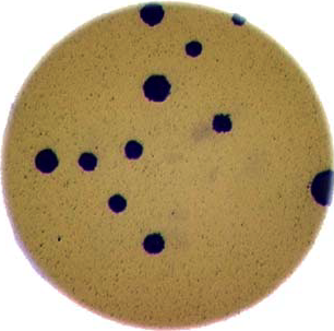
This is one of the images you will be working with in the morphometric challenge at the end of the workshop.

1. Plot and inspect the grayscale histogram of the image to determine a good threshold value for the image.
2. Create a binary mask that leaves the pixels in the bacteria colonies "on" while turning the rest of the pixels in the image "off".

Solution

Here is the code to create the grayscale histogram:

                                  image                  =                  skimage                  .                  io                  .                  imread                  (                  "../../fig/colonies01.png"                  )                  gray_image                  =                  skimage                  .                  color                  .                  rgb2gray                  (                  image                  )                  blurred_image                  =                  skimage                  .                  filters                  .                  gaussian                  (                  gray_image                  ,                  sigma                  =                  1.0                  )                  histogram                  ,                  bin_edges                  =                  np                  .                  histogram                  (                  blurred_image                  ,                  bins                  =                  256                  ,                  range                  =                  (                  0.0                  ,                  1.0                  ))                  plt                  .                  plot                  (                  bin_edges                  [                  0                  :                  -                  1                  ],                  histogram                  )                  plt                  .                  title                  (                  "Graylevel histogram"                  )                  plt                  .                  xlabel                  (                  "gray value"                  )                  plt                  .                  ylabel                  (                  "pixel count"                  )                  plt                  .                  xlim                  (                  0                  ,                  1.0                  )                  plt                  .                  show                  ()                              

The peak near one corresponds to the white image background, and the broader peak around 0.5 corresponds to the yellow/brown culture medium in the dish. The small peak near zero is what we are after: the dark bacteria colonies. A reasonable choice thus might be to leave pixels below t=0.2 on.

Here is the code to create and show the binarized image using the < operator with a threshold t=0.2:

                                  t                  =                  0.2                  binary_mask                  =                  blurred_image                  <                  t                  fig                  ,                  ax                  =                  plt                  .                  subplots                  ()                  plt                  .                  imshow                  (                  binary_mask                  ,                  cmap                  =                  'gray'                  )                  plt                  .                  show                  ()                              

When you experiment with the threshold a bit, you can see that in particular the size of the bacteria colony near the edge of the dish in the top right is affected by the choice of the threshold.

Key Points

• Thresholding produces a binary image, where all pixels with intensities above (or below) a threshold value are turned on, while all other pixels are turned off.

• The binary images produced by thresholding are held in two-dimensional NumPy arrays, since they have only one color value channel. They are boolean, hence they contain the values 0 (off) and 1 (on).

• Thresholding can be used to create masks that select only the interesting parts of an image, or as the first step before Edge Detection or finding Contours.

---

Connected Component Analysis

Overview

Teaching: 70 min
Exercises: 45 min

Questions

• How to extract separate objects from an image and describe these objects quantitatively.

Objectives

• Understand the term object in the context of images.

• Learn about pixel connectivity.

• Learn how Connected Component Analysis (CCA) works.

• Use CCA to produce an image that highlights every object in a different color.

• Characterize each object with numbers that describe its appearance.

Objects

In the thresholding episode we have covered dividing an image into foreground and background pixels. In the junk example image, we considered the colored shapes as foreground objects on a white background.

In thresholding we went from the original image to this version:

Here, we created a mask that only highlights the parts of the image that we find interesting, the objects. All objects have pixel value of True while the background pixels are False.

By looking at the mask image, one can count the objects that are present in the image (7). But how did we actually do that, how did we decide which lump of pixels constitutes a single object?

Pixel Neighborhoods

In order to decide which pixels belong to the same object, one can exploit their neighborhood: pixels that are directly next to each other and belong to the foreground class can be considered to belong to the same object.

Let's discuss the concept of pixel neighborhoods in more detail. Consider the following mask "image" with 8 rows, and 8 columns. Note that for brevity, 0 is used to represent False (background) and 1 to represent True (foreground).

            0 0 0 0 0 0 0 0 0 1 1 0 0 0 0 0 0 1 1 0 0 0 0 0 0 0 0 1 1 1 0 0 0 0 0 1 1 1 1 0 0 0 0 0 0 0 0 0                      

The pixels are organized in a rectangular grid. In order to understand pixel neighborhoods we will introduce the concept of "jumps" between pixels. The jumps follow two rules: First rule is that one jump is only allowed along the column, or the row. Diagonal jumps are not allowed. So, from a center pixel, denoted with o, only the pixels indicated with an x are reachable:

The pixels on the diagonal (from o) are not reachable with a single jump, which is denoted by the -. The pixels reachable with a single jump form the 1-jump neighborhood.

The second rule states that in a sequence of jumps, one may only jump in row and column direction once -> they have to be orthogonal. An example of a sequence of orthogonal jumps is shown below. Starting from o the first jump goes along the row to the right. The second jump then goes along the column direction up. After this, the sequence cannot be continued as a jump has already been made in both row and column direction.

All pixels reachable with one, or two jumps form the 2-jump neighborhood. The grid below illustrates the pixels reachable from the center pixel o with a single jump, highlighted with a 1, and the pixels reachable with 2 jumps with a 2.

We want to revisit our example image mask from above and apply the two different neighborhood rules. With a single jump connectivity for each pixel, we get two resulting objects, highlighted in the image with 1's and 2's.

            0 0 0 0 0 0 0 0 0 1 1 0 0 0 0 0 0 1 1 0 0 0 0 0 0 0 0 2 2 2 0 0 0 0 0 2 2 2 2 0 0 0 0 0 0 0 0 0                      

In the 1-jump version, only pixels that have direct neighbors along rows or columns are considered connected. Diagonal connections are not included in the 1-jump neighborhood. With two jumps, however, we only get a single object because pixels are also considered connected along the diagonals.

            0 0 0 0 0 0 0 0 0 1 1 0 0 0 0 0 0 1 1 0 0 0 0 0 0 0 0 1 1 1 0 0 0 0 0 1 1 1 1 0 0 0 0 0 0 0 0 0                      

Object counting (optional, not included in timing)

How many objects with 1 orthogonal jump, how many with 2 orthogonal jumps?

              0 0 0 0 0 0 0 0 0 1 0 0 0 1 1 0 0 0 1 0 0 0 0 0 0 1 0 1 1 1 0 0 0 1 0 1 1 0 0 0 0 0 0 0 0 0 0 0                          

1 jump

a) 1 b) 5 c) 2

Solution

b) 5

2 jumps

a) 2 b) 3 c) 5

Solution

a) 2

Jumps and neighborhoods

We have just introduced how you can reach different neighboring pixels by performing one or more orthogonal jumps. We have used the terms 1-jump and 2-jump neighborhood. There is also a different way of referring to these neighborhoods: the 4- and 8-neighborhood. With a single jump you can reach four pixels from a given starting pixel. Hence, the 1-jump neighborhood corresponds to the 4-neighborhood. When two orthogonal jumps are allowed, eight pixels can be reached, so the 2-jump neighborhood corresponds to the 8-neighborhood.

Connected Component Analysis

In order to find the objects in an image, we want to employ an operation that is called Connected Component Analysis (CCA). This operation takes a binary image as an input. Usually, the False value in this image is associated with background pixels, and the True value indicates foreground, or object pixels. Such an image can be produced, e.g., with thresholding. Given a thresholded image, the connected component analysis produces a new labeled image with integer pixel values. Pixels with the same value, belong to the same object. Skimage provides connect component analysis in the function skimage.measure.label(). Let us add this function to the already familiar steps of thresholding an image. Here we define a reusable Python function connected_components:

                          import              numpy              as              np              import              matplotlib.pyplot              as              plt              import              skimage.io              import              skimage.color              import              skimage.filters              import              skimage.measure              def              connected_components              (              filename              ,              sigma              =              1.0              ,              t              =              0.5              ,              connectivity              =              2              ):              # load the image                            image              =              skimage              .              io              .              imread              (              filename              )              # convert the image to grayscale                            gray_image              =              skimage              .              color              .              rgb2gray              (              image              )              # denoise the image with a Gaussian filter                            blurred_image              =              skimage              .              filters              .              gaussian              (              gray_image              ,              sigma              =              sigma              )              # mask the image according to threshold                            binary_mask              =              blurred_image              <              t              # perform connected component analysis                            labeled_image              ,              count              =              skimage              .              measure              .              label              (              binary_mask              ,              connectivity              =              connectivity              ,              return_num              =              True              )              return              labeled_image              ,              count                      

Note the new import of skimage.measure in order to use the skimage.measure.label function that performs the CCA. The first four lines of code are familiar from the Thresholding episode.

Then we call the skimage.measure.label function. This function has one positional argument where we pass the binary_mask, i.e., the binary image to work on. With the optional argument connectivity, we specify the neighborhood in units of orthogonal jumps. For example, by setting connectivity=2 we will consider the 2-jump neighborhood introduced above. The function returns a labeled_image where each pixel has a unique value corresponding to the object it belongs to. In addition, we pass the optional parameter return_num=True to return the maximum label index as count.

Optional parameters and return values

The optional parameter return_num changes the data type that is returned by the function skimage.measure.label. The number of labels is only returned if return_num is True. Otherwise, the function only returns the labeled image. This means that we have to pay attention when assigning the return value to a variable. If we omit the optional parameter return_num or pass return_num=False, we can call the function as

                              labeled_image                =                skimage                .                measure                .                label                (                binary_mask                )                          

If we pass return_num=True, the function returns a tuple and we can assign it as

                              labeled_image                ,                count                =                skimage                .                measure                .                label                (                binary_mask                ,                return_num                =                True                )                          

If we used the same assignment as in the first case, the variable labeled_image would become a tuple, in which labeled_image[0] is the image and labeled_image[1] is the number of labels. This could cause confusion if we assume that labeled_image only contains the image and pass it to other functions. If you get an AttributeError: 'tuple' object has no attribute 'shape' or similar, check if you have assigned the return values consistently with the optional parameters.

We can call the above function connected_components and display the labeled image like so:

                          labeled_image              ,              count              =              connected_components              (              "junk.jpg"              ,              sigma              =              2.0              ,              t              =              0.9              ,              connectivity              =              2              )              fig              ,              ax              =              plt              .              subplots              ()              plt              .              imshow              (              labeled_image              )              plt              .              axis              (              'off'              )              plt              .              show              ()                      

Here you might get a warning UserWarning: Low image data range; displaying image with stretched contrast. or just see an all black image (Note: this behavior might change in future versions or not occur with a different image viewer).

What went wrong? When you hover over the black image, the pixel values are shown as numbers in the lower corner of the viewer. You can see that some pixels have values different from 0, so they are not actually pure black. Let's find out more by examining labeled_image. Properties that might be interesting in this context are dtype, the minimum and maximum value. We can print them with the following lines:

                          print              (              "dtype:"              ,              labeled_image              .              dtype              )              print              (              "min:"              ,              np              .              min              (              labeled_image              ))              print              (              "max:"              ,              np              .              max              (              labeled_image              ))                      

Examining the output can give us a clue why the image appears black.

            dtype: int64 min: 0 max: 11                      

The dtype of labeled_image is int64. This means that values in this image range from -2 ** 63 to 2 ** 63 - 1. Those are really big numbers. From this available space we only use the range from 0 to 11. When showing this image in the viewer, it squeezes the complete range into 256 gray values. Therefore, the range of our numbers does not produce any visible change.

Fortunately, the skimage library has tools to cope with this situation. We can use the function skimage.color.label2rgb() to convert the colors in the image (recall that we already used the simage.color.rgb2gray() function to convert to grayscale). With skimage.color.label2rgb(), all objects are colored according to a list of colors that can be customized. We can use the following commands to convert and show the image:

                          # convert the label image to color image                            colored_label_image              =              skimage              .              color              .              label2rgb              (              labeled_image              ,              bg_label              =              0              )              fig              ,              ax              =              plt              .              subplots              ()              plt              .              imshow              (              colored_label_image              )              plt              .              axis              (              'off'              )              plt              .              show              ()                      

How many objects are in that image (15 min)

Now, it is your turn to practice. Using the function connected_components, find two ways of printing out the number of objects found in the image.

What number of objects would you expect to get?

How does changing the sigma and threshold values influence the result?

Solution

As you might have guessed, the return value count already contains the number of found images. So it can simply be printed with

                                  print                  (                  "Found"                  ,                  count                  ,                  "objects in the image."                  )                              

But there is also a way to obtain the number of found objects from the labeled image itself. Recall that all pixels that belong to a single object are assigned the same integer value. The connected component algorithm produces consecutive numbers. The background gets the value 0, the first object gets the value 1, the second object the value 2, and so on. This means that by finding the object with the maximum value, we also know how many objects there are in the image. We can thus use the np.max function from Numpy to find the maximum value that equals the number of found objects:

                                  num_objects                  =                  np                  .                  max                  (                  labeled_image                  )                  print                  (                  "Found"                  ,                  num_objects                  ,                  "objects in the image."                  )                              

Invoking the function with sigma=2.0, and threshold=0.9, both methods will print

                Found 11 objects in the image.                              

Lowering the threshold will result in fewer objects. The higher the threshold is set, the more objects are found. More and more background noise gets picked up as objects. Larger sigmas produce binary masks with less noise and hence a smaller number of objects. Setting sigma too high bears the danger of merging objects.

You might wonder why the connected component analysis with sigma=2.0, and threshold=0.9 finds 11 objects, whereas we would expect only 7 objects. Where are the four additional objects? With a bit of detective work, we can spot some small objects in the image, for example, near the left border.

For us it is clear that these small spots are artifacts and not objects we are interested in. But how can we tell the computer? One way to calibrate the algorithm is to adjust the parameters for blurring (sigma) and thresholding (t), but you may have noticed during the above exercise that it is quite hard to find a combination that produces the right output number. In some cases, background noise gets picked up as an object. And with other parameters, some of the foreground objects get broken up or disappear completely. Therefore, we need other criteria to describe desired properties of the objects that are found.

Morphometrics - Describe object features with numbers

Morphometrics is concerned with the quantitative analysis of objects and considers properties such as size and shape. For the example of the images with the shapes, our intuition tells us that the objects should be of a certain size or area. So we could use a minimum area as a criterion for when an object should be detected. To apply such a criterion, we need a way to calculate the area of objects found by connected components. Recall how we determined the root mass in the Thresholding by counting the pixels in the binary mask. But here we want to calculate the area of several objects in the labeled image. The skimage library provides the function skimage.measure.regionprops to measure the properties of labeled regions. It returns a list of RegionProperties that describe each connected region in the images. The properties can be accessed using the attributes of the RegionProperties data type. Here we will use the properties "area" and "label". You can explore the skimage documentation to learn about other properties available.

We can get a list of areas of the labeled objects as follows:

                          # compute object features and extract object areas                            object_features              =              skimage              .              measure              .              regionprops              (              labeled_image              )              object_areas              =              [              objf              [              "area"              ]              for              objf              in              object_features              ]              object_areas                      

This will produce the output

            [318542, 1, 523204, 496613, 517331, 143, 256215, 1, 68, 338784, 265755]                      

Plot a histogram of the object area distribution (10 min)

Similar to how we determined a "good" threshold in the Thresholding episode, it is often helpful to inspect the histogram of an object property. For example, we want to look at the distribution of the object areas.

1. Create and examine a histogram of the object areas obtained with skimage.measure.regionprops.
2. What does the histogram tell you about the objects?

Solution

The histogram can be plotted with

                                  fig                  ,                  ax                  =                  plt                  .                  subplots                  ()                  plt                  .                  hist                  (                  object_areas                  )                  plt                  .                  xlabel                  (                  "Area (pixels)"                  )                  plt                  .                  ylabel                  (                  "Number of objects"                  )                  plt                  .                  show                  ()                              

The histogram shows the number of objects (vertical axis) whose area is within a certain range (horizontal axis). The height of the bars in the histogram indicates the prevalence of objects with a certain area. The whole histogram tells us about the distribution of object sizes in the image. It is often possible to identify gaps between groups of bars (or peaks if we draw the histogram as a continuous curve) that tell us about certain groups in the image.

In this example, we can see that there are four small objects that contain less than 50000 pixels. Then there is a group of four (1+1+2) objects in the range between 200000 and 400000, and three objects with a size around 500000. For our object count, we might want to disregard the small objects as artifacts, i.e, we want to ignore the leftmost bar of the histogram. We could use a threshold of 50000 as the minimum area to count. In fact, the object_areas list already tells us that there are fewer than 200 pixels in these objects. Therefore, it is reasonable to require a minimum area of at least 200 pixels for a detected object. In practice, finding the "right" threshold can be tricky and usually involves an educated guess based on domain knowledge.

Filter objects by area (10 min)

Now we would like to use a minimum area criterion to obtain a more accurate count of the objects in the image.

1. Find a way to calculate the number of objects by only counting objects above a certain area.

Solution

One way to count only objects above a certain area is to first create a list of those objects, and then take the length of that list as the object count. This can be done as follows:

                                  min_area                  =                  200                  large_objects                  =                  []                  for                  objf                  in                  object_features                  :                  if                  objf                  [                  "area"                  ]                  >                  min_area                  :                  large_objects                  .                  append                  (                  objf                  [                  "label"                  ])                  print                  (                  "Found"                  ,                  len                  (                  large_objects                  ),                  "objects!"                  )                              

Another option is to use Numpy arrays to create the list of large objects. We first create an array object_areas containing the object areas, and an array object_labels containing the object labels. The labels of the objects are also returned by skimage.measure.regionprops. We have already seen that we can create boolean arrays using comparison operators. Here we can use object_areas > min_area to produce an array that has the same dimension as object_labels. It can then used to select the labels of objects whose area is greater than min_area by indexing:

                                  object_areas                  =                  np                  .                  array                  ([                  objf                  [                  "area"                  ]                  for                  objf                  in                  object_features                  ])                  object_labels                  =                  np                  .                  array                  ([                  objf                  [                  "label"                  ]                  for                  objf                  in                  object_features                  ])                  large_objects                  =                  object_labels                  [                  object_areas                  >                  min_area                  ]                  print                  (                  "Found"                  ,                  len                  (                  large_objects                  ),                  "objects!"                  )                              

The advantage of using Numpy arrays is that for loops and if statements in Python can be slow, and in practice the first approach may not be feasible if the image contains a large number of objects. In that case, Numpy array functions turn out to be very useful because they are much faster.

In this example, we can also use the np.count_nonzero function that we have seen earlier together with the > operator to count the objects whose area is above min_area.

                                  n                  =                  np                  .                  count_nonzero                  (                  object_areas                  >                  min_area                  )                  print                  (                  "Found"                  ,                  n                  ,                  "objects!"                  )                              

For all three alternatives, the output is the same and gives the expected count of 7 objects.

Using functions from Numpy and other Python packages

Functions from Python packages such as Numpy are often more efficient and require less code to write. It is a good idea to browse the reference pages of numpy and skimage to look for an availabe function that can solve a given task.

Remove small objects (20 min)

We might also want to exclude (mask) the small objects when plotting the labeled image.

1. Enhance the connected_components function such that it automatically removes objects that are below a certain area that is passed to the function as an optional parameter.

Solution

To remove the small objects from the labeled image, we change the value of all pixels that belong to the small objects to the background label 0. One way to do this is to loop over all objects and set the pixels that match the label of the object to 0.

                                  for                  object_id                  ,                  objf                  in                  enumerate                  (                  object_features                  ,                  start                  =                  1                  ):                  if                  objf                  [                  "area"                  ]                  <                  min_area                  :                  labeled_image                  [                  labeled_image                  ==                  objf                  [                  "label"                  ]]                  =                  0                              

Here Numpy functions can also be used to eliminate for loops and if statements. Like above, we can create an array of the small object labels with the comparison object_areas < min_area. We can use another Numpy function, np.isin, to set the pixels of all small objects to 0. np.isin takes two arrays and returns a boolean array with values True if the entry of the first array is found in the second array, and False otherwise. This array can then be used to index the labeled_image and set the entries that belong to small objects to 0.

                                  object_areas                  =                  np                  .                  array                  ([                  objf                  [                  "area"                  ]                  for                  objf                  in                  object_features                  ])                  object_labels                  =                  np                  .                  array                  ([                  objf                  [                  "label"                  ]                  for                  objf                  in                  object_features                  ])                  small_objects                  =                  object_labels                  [                  object_areas                  <                  min_area                  ]                  labeled_image                  [                  np                  .                  isin                  (                  labeled_image                  ,                  small_objects                  )]                  =                  0                              

An even more elegant way to remove small objects from the image is to leverage the skimage.morphology module. It provides a function skimage.morphology.remove_small_objects that does exactly what we are looking for. It can be applied to a binary image and returns a mask in which all objects smaller than min_area are excluded, i.e, their pixel values are set to False. We can then apply skimage.measure.label to the masked image:

                                  object_mask                  =                  skimage                  .                  morphology                  .                  remove_small_objects                  (                  binary_mask                  ,                  min_area                  )                  labeled_image                  ,                  n                  =                  skimage                  .                  measure                  .                  label                  (                  object_mask                  ,                  connectivity                  =                  connectivity                  ,                  return_num                  =                  True                  )                              

Using the skimage features, we can implement the enhanced_connected_component as follows:

                                  def                  enhanced_connected_components                  (                  filename                  ,                  sigma                  =                  1.0                  ,                  t                  =                  0.5                  ,                  connectivity                  =                  2                  ,                  min_area                  =                  0                  ):                  image                  =                  skimage                  .                  io                  .                  imread                  (                  filename                  )                  gray_image                  =                  skimage                  .                  color                  .                  rgb2gray                  (                  image                  )                  blurred_image                  =                  skimage                  .                  filters                  .                  gaussian                  (                  gray_image                  ,                  sigma                  =                  sigma                  )                  binary_mask                  =                  blurred_image                  <                  t                  object_mask                  =                  skimage                  .                  morphology                  .                  remove_small_objects                  (                  binary_mask                  ,                  min_area                  )                  labeled_image                  ,                  count                  =                  skimage                  .                  measure                  .                  label                  (                  object_mask                  ,                  connectivity                  =                  connectivity                  ,                  return_num                  =                  True                  )                  return                  labeled_image                  ,                  count                              

We can now call the function with a chosen min_area and display the resulting labeled image:

                                  labeled_image                  ,                  count                  =                  enhanced_connected_components                  (                  "fig/junk.jpg"                  ,                  sigma                  =                  2.0                  ,                  t                  =                  0.9                  ,                  connectivity                  =                  2                  ,                  min_area                  =                  min_area                  )                  colored_label_image                  =                  skimage                  .                  color                  .                  label2rgb                  (                  labeled_image                  ,                  bg_label                  =                  0                  )                  fig                  ,                  ax                  =                  plt                  .                  subplots                  ()                  plt                  .                  imshow                  (                  colored_label_image                  )                  plt                  .                  axis                  (                  'off'                  )                  plt                  .                  show                  ()                  print                  (                  "Found"                  ,                  count                  ,                  "objects in the image."                  )                              

                Found 7 objects in the image.                              

Note that the small objects are "gone" and we obtain the correct number of 7 objects in the image.

Color objects by area (10 min)

Finally, we would like to display the image with the objects colored according to the magnitude of their area. In practice, this can be used with other properties to give visual cues of the object properties.

Solution

We already know how to get the areas of the objects from the regionprops. We just need to insert a zero area value for the background (to color it like a zero size object). The background is also labeled 0 in the labeled_image, so we insert the zero area value in front of the first element of object_areas with np.insert. Then we can create a colored_area_image where we assign each pixel value the area by indexing the object_areas with the label values in labeled_image.

                                  object_areas                  =                  np                  .                  array                  ([                  objf                  [                  "area"                  ]                  for                  objf                  in                  skimage                  .                  measure                  .                  regionprops                  (                  labeled_image                  )])                  object_areas                  =                  np                  .                  insert                  (                  0                  ,                  1                  ,                  object_areas                  )                  colored_area_image                  =                  object_areas                  [                  labeled_image                  ]                  fig                  ,                  ax                  =                  plt                  .                  subplots                  ()                  im                  =                  plt                  .                  imshow                  (                  colored_area_image                  )                  cbar                  =                  fig                  .                  colorbar                  (                  im                  ,                  ax                  =                  ax                  ,                  shrink                  =                  0.85                  )                  cbar                  .                  ax                  .                  set_title                  (                  'Area'                  )                  plt                  .                  axis                  (                  'off'                  )                  plt                  .                  show                  ()                              

Key Points

• We can use skimage.measure.label to find and label connected objects in an image.

• We can use skimage.measure.regionprops to measure properties of labeled objects.

• We can use skimage.morphology.remove_small_objects to mask small objects and remove artifacts from an image.

• We can display the labeled image to view the objects colored by label.

---

Challenges

Overview

Teaching: 10 min
Exercises: 40 min

Questions

• What are the questions?

Objectives

• What are the objectives?

In this episode, we will provide two different challenges for you to attempt, based on the skills you have acquired so far. One of the challenges will be related to the shape of objects in images (morphometrics), while the other will be related to colors of objects in images (colorimetrics). We will not provide solution code for either of the challenges, but your instructors should be able to give you some gentle hints if you need them.

Morphometrics: Bacteria Colony Counting

As mentioned in the workshop introduction, your morphometric challenge is to determine how many bacteria colonies are in each of these images. These images can be found in the Desktop/workshops/image-processing/10-challenges/morphometric directory.

Write a Python program that uses skimage to count the number of bacteria colonies in each image, and for each, produce a new image that highlights the colonies. The image should look similar than this one:

Additionally, print out the number of colonies for each image.

Colorimetrics: titration color analysis

The video showing the titration process first mentioned in the workshop introduction episode can be found in the Desktop/workshops/image-processing/10-challenges/colorimetric directory. Write a Python program that uses skimage to analyze the video on a frame-by-frame basis. Your program should do the following:

1. Sample a kernel from the same location on each frame, and determine the average red, green, and blue channel value.

2. Display a graph plotting the average color channel values as a function of the frame number, similar to this image:

   

3. Save the graph as an image named titration.png.

4. Output a CSV file named titration.csv, with each line containing the frame number, average red value, average green value, and average blue value

Key Points

• What are the key points?

---

Tkinter Increase Drawing Speed Images

Source: https://datacarpentry.org/image-processing/aio/index.html

Share :