Write a Program to Create a Graph in Java Where Actors and Actresses Are Nodes
CS 10: Winter 2016
Lecture 19, February 15
Breadth-first search on a graph
One question we might ask about a graph is how few edges we need to traverse to find a path from one vertex to another. In other words, assuming that some path exists from vertex x to vertex y , find a path from x to y that has the fewest edges.
One application is the famous Kevin Bacon game, which you will implement in Lab Assignment 5. Consider a movie actor, say Renée Adorée, a silent film actress from the 1920s. She appeared in a film with Bessie Love, who made a movie with Eli Wallach, who acted in a film with Kevin Bacon, and so we say that Renée Adorée's "Kevin Bacon number" is 3. If we were to make a graph where the vertices represent actors and we put an edge between vertices if their actors ever made a movie together, then we can use breadth-first search to find anyone's Kevin Bacon number: the minimum number of actors between a given actor and Kevin Bacon.
I'll describe breadth-first search, which we abbreviate as BFS, for you, but I'll give you no code. That's because you'll be implementing BFS in Lab Assignment 5.
We perform BFS from a given start vertex s . We sometimes call s the root vertex. We can either designate a specific goal vertex, or we can just search to all vertices that are reachable from the start vertex (i.e., there exist paths from the start vertex to the vertices). We want to determine, for each vertex x that the search encounters, an unweighted shortest path from s to x , that is, a path from s to x with the minimum length (fewest edges). Later in the course, when we consider weighted graphs, we'll extend the notion of shortest paths to account for edge weights.
We usually record two pieces of information about each vertex x :
-
The length of an unweighted shortest path from s to x , as the number of edges.(This is optional in many applications, including the Kevin Bacon game.)
-
A back-pointer from x , which is the vertex that immediately precedes x on a shortest path from s to x . For example, let's look at that graph again:
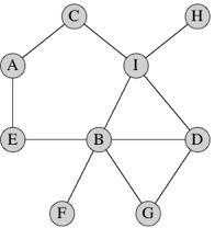
In this graph, an unweighted shortest path from vertex D to vertex A is D, I, C, A, and so A would have a back-pointer to C, C would have a back-pointer to I, and I would have a back-pointer to D. Because vertex D is the start vertex, no vertex precedes it. We can say that its back-pointer is
null(depending on the type of the back-pointer), or we can say that D is its own back-pointer, so that a vertex that is its own back-pointer must be the start vertex.This unweighted shortest path is not unique in this graph. Another unweighted shortest path from vertex D to vertex A is D, B, E, A. In this path, A would have a back-pointer to E, E would have a back-pointer to B, B would have a back-pointer to D, and D's back-pointer would be
None.
One way to think of BFS in terms of sending waves of runners over the graph in discrete timesteps. We'll focus on undirected graphs. I'll call the start vertex s , and at first I won't designate a goal vertex.
- Record the "distance" from the start vertex s to itself as 0, and record the back-pointer for s as
null. - At time 0, send out runners from s by sending out one runner over each edge incident on s . (So that the number of runners sent out at time 0 equals the degree of s .)
- Each runner arrives at a vertex adjacent to s at time 1. For each of these vertices, record its distance from s as 1 and its back-pointer as s .
- At time 1, send out runners from each vertex whose distance from s is 1. As we did with s at time 0, send out one runner along each edge from each of these vertices.
- Each runner will arrive at another vertex at time 2. Let's say that the runner left vertex x at time 1 and arrives at vertex y at time 2. Vertex y could have already been visited by a runner (perhaps it is s or perhaps it is another vertex that was visited at time 1). Or vertex y might not have been visited before. If vertex y had already been visited, forget about it; we already know its distance from s and its back-pointer. But if vertex y had not already been visited, record its distance from s as 2, and record its back-pointer as x (the vertex that the runner came from).
- At time 2, send out runners from each vertex whose distance from s is 2. As before, send out one runner along each edge from each of these vertices.
- Each runner will arrive at another vertex at time 3. If the vertex has been visited before, forget about it. Otherwise, record its distance from s as 3, and record its back-pointer as the vertex from which the runner came.
- Continue in this way until all vertices that are reachable from the start vertex have been visited.
If there is a specific goal vertex, you can stop this process once it has been visited.
In the above graph, let's designate vertex D as the start vertex, so that D's distance is 0 and its back-pointer is null. At time 1, runners visit vertices G, B, and I, and so each of these vertices gets a distance of 1 and D as their back-pointers. At time 2, runners from G, B, and I visit vertices D, G, B, I, F, E, C, and H. D, G, B, and I have already been visited, but F, E, C, and H all get a distance of 2. F and E get B as their back-pointer, and C and H get I as their back-pointer. At time 3, runners from F, E, C, and H visit vertices B, A, and I. B and I have already been visited, but A gets a distance of 3, and its back-pointer is set arbitrarily to either of E and C (it doesn't matter which, since either E or C precedes A on an unweighted shortest path from D). Now all vertices have been visited, and the breadth-first search terminates.
To determine the vertices on a shortest path, we use the back-pointers to get the vertices on a shortest path in reverse order. (But you know how easy it is to reverse a list, and sometimes you're fine with knowing the path in reverse order, such as when you want to display it.) Let's look at the vertices on an unweighted shortest path from D to A. We know that A is reachable from D because it has a back-pointer. So A is on the path, and it is preceded by its back-pointer. Let's say that A's back-pointer is E (which I chose arbitrarily over C so that I wouldn't get a reversed path that spells "ACID"). So E is the next vertex on the reversed path. E's back-pointer is B, and so B is the next vertex on the reversed path. B's back-pointer is D, and so D is the next vertex on the reversed path. D's back-pointer is null, and so we are done constructing the reversed path: it contains, in order, vertices A, E, B, and D.
Implementing BFS
You can't implement BFS by following the above description exactly. That's because you can't send out lots of runners at exactly the same time. You can do only one thing at a time, and so you couldn't send runners out along all edges incident on vertices G, B, and I all at the same time. You need to simulate doing that by sending out one runner at a time.
Let's define the frontier of the BFS as the set of vertices that have been visited by runners but have yet to have runners leave them. If you send out runners one at a time, at any moment, the vertices in the frontier are all at either some distance i or distance i + 1 from the start vertex. For example, suppose that we have sent out runners from vertices D, G, and B so that they are no longer in the frontier. The frontier consists of vertex I, at distance 1, and vertices F and E, at distance 2.
One key to implementing BFS is to treat the frontier properly. In particular, you want to maintain it as a FIFO queue.
Here is "pseudocode" (i.e., not real Java code) for BFS:
queue = new Queue(); queue.enqueue(s); // initialize the queue to contain only the start vertex s distance of s = 0; while (!queue.isEmpty()) { x = queue.dequeue(); { // remove vertex x from the queue for (each vertex y that is adjacent to x) { if (y has not been visited yet) { y's distance = x's distance + 1; y's back-pointer = x; queue.enqueue(y); // insert y into the queue } } } One property of BFS is that at any time, the distances of vertices on the queue are all either d or d + 1, for some nonnegative integer d , with all the vertices at distance d preceding those at distance d + 1. We can show this property by induction on the number of enqueue and dequeue operations. (You will not be asked about this proof on the final.) Anyone still reading? At first, we have just one vertex on the queue, and its distance is 0. Now let's consider the two operations, with dequeue first. If the property holds before dequeueing, then surely removing a vertex from the queue cannot cause a vioation. Now let's consider enqueueing. Suppose that the most recently dequeued vertex had distance d . Because we assume that the property holds, after dequeueing, the first vertex in the queue must have distance d or d + 1. Any vertex enqueued has distance d + 1 (1 greater than the distance of the dequeued vertex), and because enqueued vertices follow all others in the queue, the property holds after enqueueing.
Now we have a couple more questions to answer:
- How do we represent the distance and back-pointer for each vertex?
- How do we know whether a vertex has been visited?
Representing vertex information
Again, you have a couple of choices. If you create a class, say Vertex, to represent what you need to know about a vertex, it can have whatever instance variables you like. So a Vertex object could have instance variables distance, backPointer, and even visited. Of course, you could make visited unnecessary by initializing distance to -1 and saying that the vertex has been visited only if its distance variable is not -1. In Lab Assignment 5, you do not necessarily need to keep track of distances.
This approach is nice because it encapsulates what you'd like to know about a vertex within its object. But this approach has a downside: you need to initialize the instance variables for every vertex before you commence send out runners from the start vertex. You wouldn't want to use, say, the visited value from a previous BFS, right? Ditto for the distance value.
There's another way: use a Map. If you want to store back-pointers, store them in a Map, where the key is a reference to a Vertex object and the value is a reference to the Vertex object for its immediate predecessor on an unweighted shortest path from the start vertex. You can use this same Map to record whether a vertex has been visited, because you can say that a vertex has been visited if and only if its Vertex object appears in the Map. You can use the containsKey method from the Map interface to determine whether the Map contains a reference to particular Vertex object. The beauty of using a Map is that initializing is E-Z: just make a new Map. There is one other detail you need to take care of: the start vertex. It has no predecessor, but you want to record that it has been visited initially. So you'll need to store a reference to its Vertex object in the Map, and you can just use null as the corresponding value.
There is yet another way: store the breadth-first tree as a separate directed graph. This is also called a shortest-path tree. This is what we want you to do on Lab 5. Each directed edge (u,v) is equivalent to u 's back-pointer being v . Looked at another way, each directed edge is oriented on a path toward the start vertex. Every vertex has at most one leaving edge in a breadth-first tree, since every vertex has at most one back-pointer. The way to tell if a vertex has been visited is to see if it has been added to this shortest-path tree.
How long does BFS take? We visit each vertex and each edge at most once. For a graph with n vertices and m edges, the running time is O(n +m).
Depth-first search
You can think of BFS like a "layered" search, where we visit the start vertex at distance 0, then the next "layer" of vertices at distance 1, then the next layer at distance 2, and so on. We really need the queue to keep track of which vertex we search from next.
Instead, you can search the graph as if it were a maze. That's depth-first search, or DFS. You keep going deeper and deeper in the maze, making choices at the various forks in the road, until you hit a dead-end. Then you back up to one of the choice points and make a different choice. If you're fairy-tale clever, you'll scatter some bread crumbs behind you, so that you can see if you've come back to the same point and are just walking in circles. Then you'd want to do the same thing as if you hit a dead end.
Whereas BFS keeps track of vertices on a queue, DFS uses a stack. We can either use our own stack, or take advantage of the run-time stack and write DFS recursively. If we use our own stack the code above almost works for DFS, with the stack replaced by a queue, enqueue replaced by push, and dequeue replaced by pop. We do have to be careful about how we define "visited." For DFS a vertex becomes visited when it is popped off of the stack, not when it is pushed onto the stack. So we don't want to record the distance and back pointer until we pop the vertex. The same would also work for BFS, but because a queue is FIFO the nodes come out of the queue in the order that they entered it. Therefore we might as well visit the node when we first discover it and avoid enqueuing the same vertex multiple times.
I prefer to use the run-time stack, because I find recursive code more natural to understand than maintaining a data structure. So here is recursive pseudocode for DFS:
visit(s); void visit(u) { do whatever it means to start a visit of u; for (each vertex v that is adjacent to u) if (v has not been visited yet) visit(v); do whatever it means to finish a visit of u; } Now, we can use a Set to keep track of which vertices have been visited. Or we can record depth-first distances, but they're not very interesting.
What's more interesting are discovery times times and finishing times for vertices. Keep a static integer time, and when we start or finish a visit of a vertex, record the current value of time and then increment time:
time = 0; visit(s); void visit(u) { u's discovery time = time; time++; for (each vertex v that is adjacent to u) if (v has not been visited yet) visit(v); u's finishing time = time; time++; } I'll go through an example in class.
If the graph is not connected it is possible that some vertices will not be reached by running BFS or DFS. In fact, the standard way to determine if a graph is connected is to run one of these algorithms from an arbitrary vertex and see if all vertices get visited. Usually if BFS does not reach all the vertices we will ignore those which are not reached. (Or in the case of the Kevin Bacon game, we say that their Bacon numbers are infinite.) But for many applications of DFS it is better to pick an arbitrary unvisited vertex as the new start vertex and call visit again. However, do not reset time to 0.
Like BFS, DFS visits each vertex and edge at most once, and so its running time is O(n +m).
Why are discovery and finishing times helpful? For one thing, we can use them to perform a topological sort of a directed acyclic graph.
Topological sorting
A directed graph is acyclic if it contains no directed cycles. We call a directed acyclic graph a dag. Sometimes, we want to find a linear order of the vertices of a dag such that all edges in the dag go in the direction of the linear order. That is a topological sort of the dag. For example, if we order all the vertices from left to right, then all directed edges should go from left to right.
Here's a dag that represents dependencies for putting on goalie equipment in ice hockey:
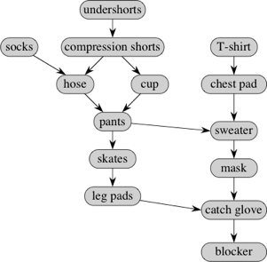
An edge (u,v) indicates that you have to put on article u before putting on article v . For example, the edge from chest pad to sweater says that you have to put on the chest pad before the sweater. On the other hand, some articles have no particular relative order. For example, it doesn't matter whether you put on compression shorts before or after the T-shirt.
You can put on only one article at a time, and so you'd like to find a linear order so that you don't have to undo having put on one article in order to put on another. In other words, you'd like to topologically sort this dag of goalie gear. Here's one possible order, given by the numbers next to the vertices:
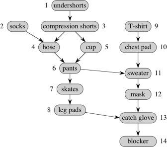
So undershorts would go on first, then socks, compression shorts, hose, cup, pants, skates, leg pads, T-shirt, chest pad, sweater, mask, catch glove, and finally the blocker. That's not the only possible order. Here's another: T-shirt, socks, chest pad, undershorts, compression shorts, cup, hose, pants, sweater, mask, skates, leg pads, catch glove, blocker.
Here is an incredibly simple algorithm to topologically sort a dag:
- Run DFS on the dag to compute the finishing times for all vertices.
- As each vertex is finished, insert it onto the front of a linked list.
- The linked list contains the topologically sorted vertices, in order.
This algorithm runs in O(n +m) time. Why? Step 1, DFS, takes O(n +m) time. Step 2, inserting each vertex onto the front of a linked list, takes constant time per vertex, or O(n) time altogether. Step 3 is really just saying that the result of step 2 is the answer. So the entire algorithm takes O(n +m) time.
I'll go through an example for the goalie-gear dag in class.
Other applications of DFS
There are may other applications of DFS that you will learn if you take CS 31, our Algorithms course. The book presents a lot of problems that can be solved by DFS - reachability, strongly connected components, transitive closure, and topological sorting. Many of these require classifying edges into groups.
For an undirected graph edges can be broken into two groups: discovery edges and back edges. Discovery edges are the first edge to find a vertex. They form a tree, the DFS tree. Back edges go back up the tree to an ancestor, and indicate that a cycle exists in the graph. For directed graphs it becomes a bit more complicated - there are also forward edges that connect a node to a descendent in the DFS tree and cross edges that connect two nodes, neither of which is the ancestor of the other.
However, the book does not mention the culmination of "everything that can be done with DFS." That is graph planarity. Bob Tarjan developed an amazing Θ(n + m) time algorithm for determining if a graph is planar (can be drawn on a plane with no crossing edges) using DFS.
Write a Program to Create a Graph in Java Where Actors and Actresses Are Nodes
Source: https://www.cs.dartmouth.edu/~scot/cs10/lectures/19/19.html